Chapter 2 Neuralnet Package

#install.packages("neuralnet")
rm(list=ls())
library(neuralnet)

2.1 Example 1 - Boston

library(MASS)
rm(list=ls())
data(Boston)

2.1.1 Scale, Training and Test Datasets

Boston.st = scale(Boston)
set.seed(1)
index <- sample(1:nrow(Boston.st),round(0.8*nrow(Boston.st)))
trainBoston.st <- Boston.st[index,]
testBoston.st <- Boston.st[-index,]

2.1.2 Build model

set.seed(1)
neuralnetmodel = neuralnet(medv~crim+nox, data = trainBoston.st, 
                           linear.output = TRUE, 
                           act.fct = "logistic",
                           hidden = c(2))

plot(neuralnetmodel)

neuralnetmodel$weights

## [[1]]
## [[1]][[1]]
##            [,1]      [,2]
## [1,]  -38.34128  5.724901
## [2,]   20.11112 -3.802220
## [3,] -122.96637 -2.323184
## 
## [[1]][[2]]
##            [,1]
## [1,] -1.4262287
## [2,]  0.6035351
## [3,]  1.3660896

neuralnetmodel$err.fct

## function (x, y) 
## {
##     1/2 * (y - x)^2
## }
## <bytecode: 0x000000001c462b10>
## <environment: 0x000000001c461488>
## attr(,"type")
## [1] "sse"

neuralnetmodel$act.fct

## function (x) 
## {
##     1/(1 + exp(-x))
## }
## <bytecode: 0x000000001c45c288>
## <environment: 0x000000001c45b990>
## attr(,"type")
## [1] "logistic"

2.1.3 Get the predictions train set

train.st.y.predict = predict(neuralnetmodel,trainBoston.st)
head(train.st.y.predict, 3)

##            [,1]
## 505 -0.06150515
## 324  0.54309902
## 167 -0.06612987

1/2*(sum((trainBoston.st[,"medv"]-as.numeric(train.st.y.predict))^2))

## [1] 153.874

#[1] 153.874

average.error.train = 1/(405)*(sum((trainBoston.st[,"medv"]-as.numeric(train.st.y.predict))^2))
average.error.train

## [1] 0.7598714

153.874*2/405

## [1] 0.7598716

2.1.4 Get the predictions test set

test.st.y.predict = predict(neuralnetmodel,testBoston.st)
head(test.st.y.predict, 3)

##          [,1]
## 6  0.54326440
## 7 -0.06064561
## 9 -0.06067375

1/2*(sum((testBoston.st[,"medv"]-as.numeric(test.st.y.predict))^2))

## [1] 22.56024

#[1] 22.56024

average.error.test = 1/(101)*(sum((testBoston.st[,"medv"]-as.numeric(test.st.y.predict))^2))
average.error.test

## [1] 0.4467374

2.1.5 Forward propagation

head(trainBoston.st[,c("crim","nox","medv")])

##            crim        nox        medv
## 505 -0.40736095  0.1579678 -0.05793197
## 324 -0.38709366 -0.5324154 -0.43848654
## 167 -0.18640065  0.4341211  2.98650460
## 129 -0.38226778  0.5980871 -0.49285148
## 418  2.59570533  1.0727255 -1.31919854
## 471  0.08548074  0.2183763 -0.28626471

trainBoston.st[1,c("crim","nox","medv")]

##        crim         nox        medv 
## -0.40736095  0.15796779 -0.05793197

Z1_2 = sum(neuralnetmodel$weights[[1]][[1]][,1]*c(1,trainBoston.st[1,c("crim","nox")]))
Z1_2

## [1] -65.95849

a1_2 = 1/(1+exp(-Z1_2))
a1_2

## [1] 2.26251e-29

Z2_2 = sum(neuralnetmodel$weights[[1]][[1]][,2]*c(1,trainBoston.st[1,c("crim","nox")]))
Z2_2

## [1] 6.906789

a2_2 = 1/(1+exp(-Z2_2))
a2_2

## [1] 0.999

Z1_3 = sum(neuralnetmodel$weights[[1]][[2]][,1]*c(1,a1_2,a2_2))

a1_3=Z1_3
a1_3

## [1] -0.06150515

2.1.6 Model Tuning

Although these seem like good results this may simply be a result of the subseted training and testing data so it is important to test the model performance further. In this example I will perform k-fold cross validation using 10 folds (10 fold cross validation)

get the validation indeces using the createFolds function provided by the

caret package

#install.packages("caret")
library(caret)

## Loading required package: lattice

## Loading required package: ggplot2

## Warning: replacing previous import 'vctrs::data_frame' by 'tibble::data_frame'
## when loading 'dplyr'

set.seed(1)
folds <- createFolds(trainBoston.st[,"medv"], k = 10)
#results is a vector that will contain the average sum error square for each 
# of the network trainings for the validation set.

#errors.cv.number.of.neurons <- c()

#for (hidden in 1:2){
errors.cv.validation <- c()
for (fld in folds){
  
  #train the network (note I have subsetted out the indeces in the validation set)
  set.seed(1)
  neuralnetmodel <- neuralnet(medv~crim+nox, data = trainBoston.st[-fld,], 
                  linear.output = TRUE, 
                  act.fct = "logistic",
                  hidden = c(2))
  
  #get the predictions from the network for the validation set
  yhat.fld <- predict(neuralnetmodel, trainBoston.st[fld,])
  
  errorsq.fld = (trainBoston.st[fld,"medv"]-
                                                as.numeric(yhat.fld))^2
  
  errors.cv.validation <- c(errors.cv.validation, errorsq.fld)
} 

#errors.cv.number.of.neurons[hidden] = 

sum(errors.cv.validation)/dim(trainBoston.st)[1]

## [1] 0.7712774

2.2 Example 2 - Iris Dataset

rm(list=ls())

set.seed(1)
index <- sample(1:nrow(iris),round(0.8*nrow(iris)))
trainiris <- iris[index,]
testiris <- iris[-index,]

set.seed(1)
neuralnetmodel = neuralnet(Species~Petal.Length+Petal.Width, data = trainiris, 
                           linear.output = FALSE, 
                           act.fct = "logistic",
                           hidden = c(2), err.fct = "ce")
# stepmax = 1000000, threshold = 0.001, rep = 10 values can be changed as well.

plot(neuralnetmodel)

neuralnetmodel$weights

## [[1]]
## [[1]][[1]]
##           [,1]       [,2]
## [1,]  9.189152 -124.80564
## [2,] -1.436100   33.13635
## [3,] -1.300787   52.19249
## 
## [[1]][[2]]
##            [,1]      [,2]       [,3]
## [1,]   -2.83673 -38.59970   4.022241
## [2,]   39.67766  28.62683 -28.834230
## [3,] -113.70312  24.75467   9.921314

neuralnetmodel$err.fct

## function (x, y) 
## {
##     -(y * log(x) + (1 - y) * log(1 - x))
## }
## <bytecode: 0x000000001c4622f8>
## <environment: 0x0000000024577c00>
## attr(,"type")
## [1] "ce"

neuralnetmodel$act.fct

## function (x) 
## {
##     1/(1 + exp(-x))
## }
## <bytecode: 0x000000001c45c288>
## <environment: 0x00000000245ce3f8>
## attr(,"type")
## [1] "logistic"

train.iris.predict = predict(neuralnetmodel, trainiris)
head(round(train.iris.predict,3), 3)

##     [,1] [,2] [,3]
## 68     0    1    0
## 129    0    0    1
## 43     1    0    0

maxprobability <- apply(train.iris.predict, 1, which.max) 
train.iris.predict.class <- c('setosa', 'versicolor', 'virginica')[maxprobability] 
head(train.iris.predict.class)

## [1] "versicolor" "virginica"  "setosa"     "setosa"     "versicolor"
## [6] "versicolor"

table(train.iris.predict.class, trainiris$Species) 

##                         
## train.iris.predict.class setosa versicolor virginica
##               setosa         39          0         0
##               versicolor      0         36         2
##               virginica       0          2        41

mean(train.iris.predict.class== trainiris$Species)*100

## [1] 96.66667

test.iris.predict = predict(neuralnetmodel, testiris)
head(round(train.iris.predict,3), 3)

##     [,1] [,2] [,3]
## 68     0    1    0
## 129    0    0    1
## 43     1    0    0

maxprobability <- apply(test.iris.predict, 1, which.max) 
test.iris.predict.class <- c('setosa', 'versicolor', 'virginica')[maxprobability] 
head(test.iris.predict.class)

## [1] "setosa" "setosa" "setosa" "setosa" "setosa" "setosa"

table(test.iris.predict.class, testiris$Species) 

##                        
## test.iris.predict.class setosa versicolor virginica
##              setosa         11          0         0
##              versicolor      0         12         2
##              virginica       0          0         5

mean(test.iris.predict.class== testiris$Species)*100

## [1] 93.33333

2.2.1 Model Tuning

Get the validation indices using the createFolds function provided by the caret package

set.seed(1)
folds <- createFolds(iris$Species, k = 10)
#results is a vector that will contain the accuracy for each of the network trainings and testing
results <- c()
for (fld in folds){
  #train the network
  set.seed(1)
  nn <- neuralnet(Species~Petal.Length+Petal.Width, data = iris[-fld,],
                  hidden = c(2), err.fct = "ce", act.fct = "logistic",
                  linear.output = FALSE, stepmax = 1000000)
  
  #get the classifications from the network
  classes <- predict(nn, iris[fld,])
  maxprobability <- apply(classes, 1, which.max) 
  valid.iris.predict.class <- c('setosa', 'versicolor', 'virginica')[maxprobability] 
  
  results <- c(results, valid.iris.predict.class== iris[fld,"Species"])
} 

results

##   [1]  TRUE  TRUE  TRUE  TRUE  TRUE  TRUE  TRUE  TRUE  TRUE  TRUE  TRUE  TRUE
##  [13]  TRUE  TRUE  TRUE  TRUE  TRUE  TRUE  TRUE  TRUE  TRUE  TRUE  TRUE  TRUE
##  [25]  TRUE  TRUE  TRUE  TRUE  TRUE  TRUE  TRUE  TRUE  TRUE  TRUE  TRUE  TRUE
##  [37]  TRUE  TRUE  TRUE  TRUE FALSE  TRUE  TRUE  TRUE  TRUE  TRUE  TRUE  TRUE
##  [49]  TRUE  TRUE  TRUE FALSE  TRUE  TRUE  TRUE  TRUE  TRUE  TRUE  TRUE  TRUE
##  [61]  TRUE  TRUE  TRUE  TRUE  TRUE  TRUE FALSE  TRUE  TRUE  TRUE  TRUE  TRUE
##  [73]  TRUE  TRUE  TRUE  TRUE  TRUE  TRUE  TRUE  TRUE  TRUE  TRUE  TRUE  TRUE
##  [85]  TRUE  TRUE  TRUE  TRUE FALSE  TRUE  TRUE  TRUE  TRUE  TRUE  TRUE  TRUE
##  [97]  TRUE  TRUE FALSE  TRUE  TRUE  TRUE FALSE  TRUE  TRUE  TRUE  TRUE  TRUE
## [109]  TRUE  TRUE  TRUE  TRUE  TRUE  TRUE  TRUE  TRUE  TRUE  TRUE  TRUE  TRUE
## [121]  TRUE  TRUE  TRUE  TRUE  TRUE  TRUE  TRUE  TRUE  TRUE  TRUE  TRUE  TRUE
## [133]  TRUE  TRUE  TRUE  TRUE  TRUE  TRUE  TRUE  TRUE  TRUE  TRUE  TRUE  TRUE
## [145]  TRUE  TRUE  TRUE  TRUE  TRUE  TRUE

sum(results)/length(results)

## [1] 0.96

You can label chapter and section titles using {#label} after them, e.g., we can reference Chapter 2. If you do not manually label them, there will be automatic labels anyway, e.g., Chapter 4.

Figures and tables with captions will be placed in figure and table environments, respectively.

par(mar = c(4, 4, .1, .1))
plot(pressure, type = 'b', pch = 19)

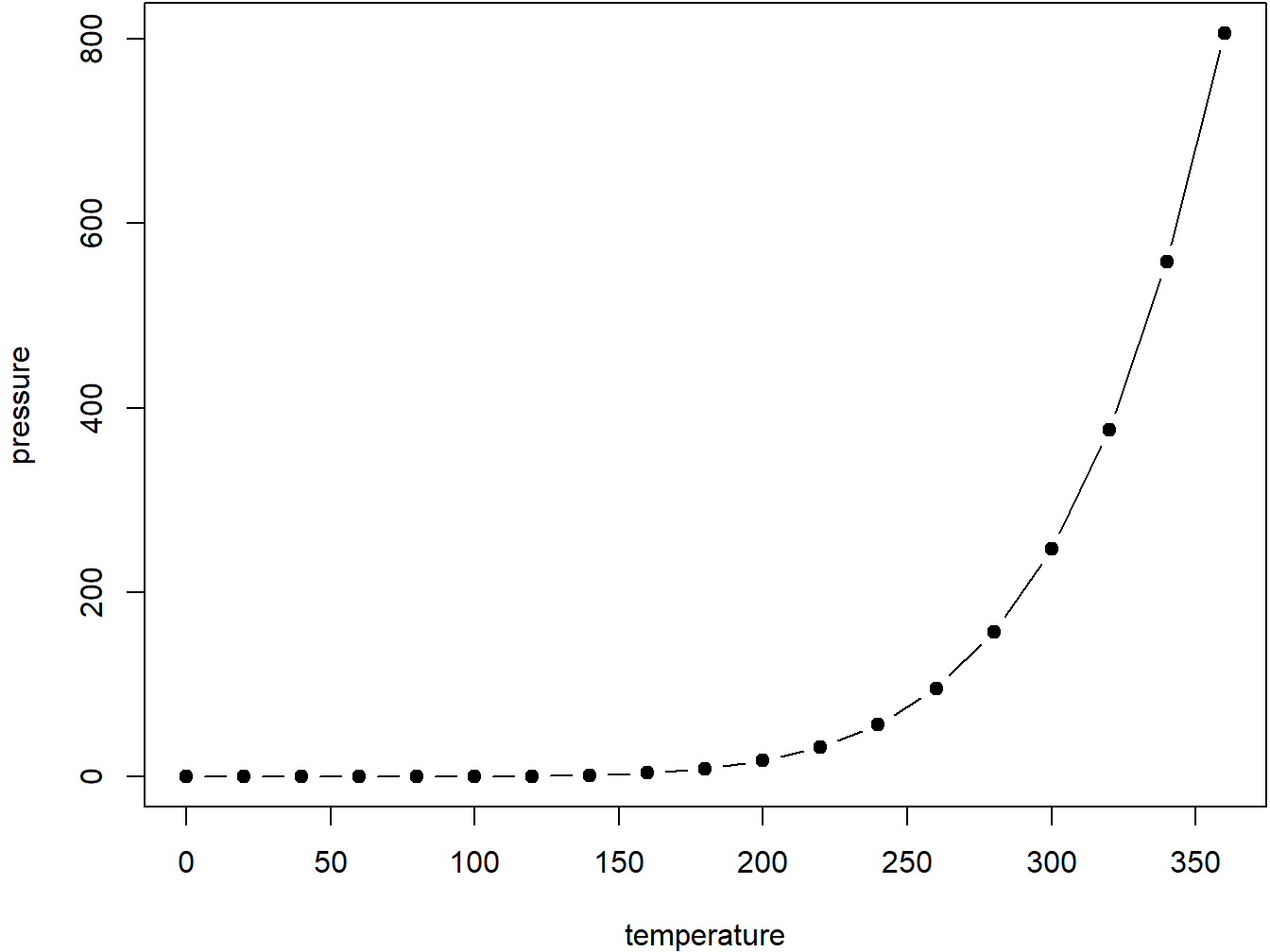
Figure 2.1: Here is a nice figure!

Reference a figure by its code chunk label with the fig: prefix, e.g., see Figure 2.1. Similarly, you can reference tables generated from knitr::kable(), e.g., see Table 2.1.

knitr::kable(
  head(iris, 20), caption = 'Here is a nice table!',
  booktabs = TRUE
)

Table 2.1: Here is a nice table!

Sepal.Length	Sepal.Width	Petal.Length	Petal.Width	Species
5.1	3.5	1.4	0.2	setosa
4.9	3.0	1.4	0.2	setosa
4.7	3.2	1.3	0.2	setosa
4.6	3.1	1.5	0.2	setosa
5.0	3.6	1.4	0.2	setosa
5.4	3.9	1.7	0.4	setosa
4.6	3.4	1.4	0.3	setosa
5.0	3.4	1.5	0.2	setosa
4.4	2.9	1.4	0.2	setosa
4.9	3.1	1.5	0.1	setosa
5.4	3.7	1.5	0.2	setosa
4.8	3.4	1.6	0.2	setosa
4.8	3.0	1.4	0.1	setosa
4.3	3.0	1.1	0.1	setosa
5.8	4.0	1.2	0.2	setosa
5.7	4.4	1.5	0.4	setosa
5.4	3.9	1.3	0.4	setosa
5.1	3.5	1.4	0.3	setosa
5.7	3.8	1.7	0.3	setosa
5.1	3.8	1.5	0.3	setosa

You can write citations, too. For example, we are using the bookdown package (Xie 2020) in this sample book, which was built on top of R Markdown and knitr (Xie 2015).

References

Xie, Yihui. 2015. Dynamic Documents with R and Knitr. 2nd ed. Boca Raton, Florida: Chapman; Hall/CRC. http://yihui.org/knitr/.

Xie, Yihui. 2020. Bookdown: Authoring Books and Technical Documents with R Markdown. https://CRAN.R-project.org/package=bookdown.