plot(sf::st_geometry(columbus))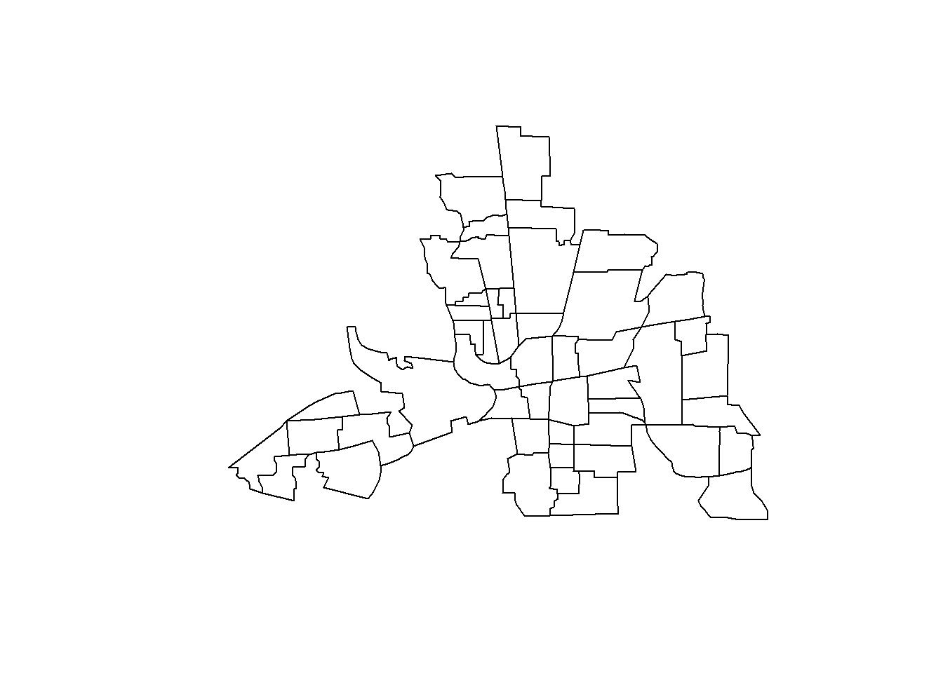
library(tmap)
tm_shape(columbus) + tm_polygons()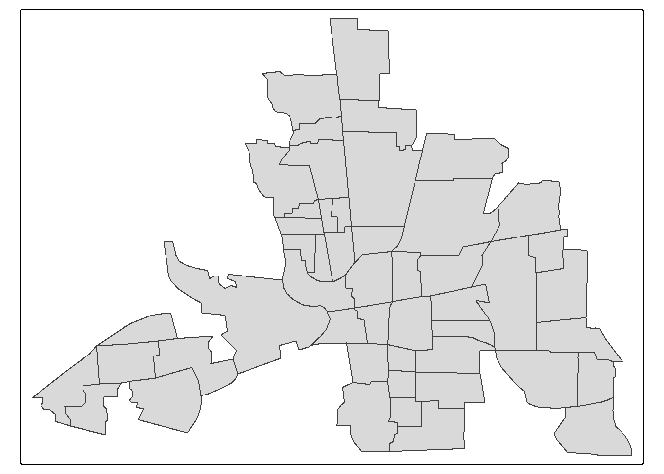
Chapter 3 - Spatial Lattice Data I
Original slide title: Applied Spatial Data Analysis — Spatial Lattice Data I. Dr. Şebnem Er, Department of Statistical Sciences, University of Cape Town.
For general spatial data handling in R using simple features (sf).
Required reading: Chapter 10.
[1] Anselin , Luc, (1999). Spatial Econometrics: Methods and Models. Luwer Academic Publishers.
[2] Arbia , Giuseppe, (2014). A Primer for Spatial Econometrics : With Applications in R. Palgrave Macmillan UK. (available at UCT library online resource)
[3] Elhorst , Paul. J. (2014). Spatial Econometrics : From Cross-Sectional Data to Spatial Panels. Springer Berlin
[4] Gelfand, A.E., Diggle, P., Guttorp , P., Fuentes, M. and Fitzmaurice, G. (2010). Handbook of Spatial Statistics. Chapman & Hall/CRC. (available at UCT library online resource) Brilliant resource to have. Part 4 is dedicated to SPPs. *
[6] Haining , Robert, (2004). Spatial Data Analysis, Theory and Practice. Cambridge University Press. *
[7] https://geodacenter.github.io/
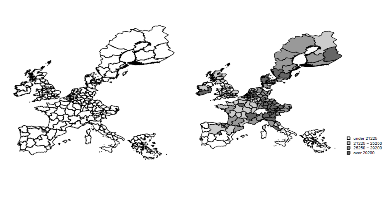
Throughout these lectures we use the Boston house-price data, Columbus crime data, and EU regional data collected at NUTS 2 level.
A spatial data set includes the geometry of the spatial units, spatial coordinates or other spatial indexing information, and the attributes associated with each unit. These attributes may include economic, demographic, social, environmental, or other variables.
The three example data sets illustrate the same lattice-data idea: each observation belongs to a spatial unit, and each unit has both geometry and attributes. The geometry lets us construct neighbourhood relationships; the attributes are the variables we analyse.
A major pleasure in working with spatial data is their visualisation. Maps are amongst the most compelling graphics.
The Columbus data provide a spatially referenced example used throughout the lecture.
plot(sf::st_geometry(columbus))
library(tmap)
tm_shape(columbus) + tm_polygons()
Plot of Crime Variable
tm_shape(columbus) + tm_polygons(style="quantile", col = "CRIME") +
  tm_legend(outside = TRUE, text.size = .8)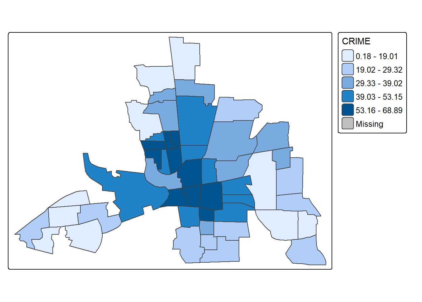
EU NUTS 2 level GDP per capita (Euros), 2009.
Tobler’s first law of geography:
“Everything is related to everything else, but close things are more related than things that are far apart.”
From this definition, we need to identify:
For each unit we therefore need a list of neighbours and a corresponding set of spatial weights.
Spatial dependence in a collection of sample observations refers to the fact that an observation associated with location \(i\) depends on observations at locations \(j\), where \(i\neq j\).
Why does spatial dependence occur? Two main reasons are highlighted by LeSage (1998, pp. 4–5):
Spatial dependence reflects a situation where values observed in one areal unit, depend on the values of neighbouring observations at near-by areas.
Positive spatial dependence
Objects—points, areas, or lines—that are close in space tend to assume similar values. This produces spatial clustering of similar values.
Negative spatial dependence
Objects that are close in space tend to assume dissimilar values. This can produce an alternating or checkerboard-like arrangement.
Spatial dependence can therefore take the form of spatial correlation.
Ref: Giuseppe Arbia lecture notes, SEAI 2011.
The level of spatial dependence can be explored using graphical techniques and statistical measures:
Cliff and Ord (1972, 1975, 1981) found Moran’s \(I\) to be a particularly useful measure in many settings.
Moran’s I and Geary’s C are very alike, and they both account for the attribute similarity and locational similarity. Moran’s I looks at similarity, whereas Geary’s C focuses on dissimilarity, similar to the notion of variogram as in geostatistics. Moran’s I and Geary’s C are interpreted in an opposite manner. Moran’s I and Geary’s C are very much linked to weights matrices. With correlograms and variograms, we will step away from weights matrices and look at distances. We still have attribute similarity however the locational similarity will be replaced with increasing distances between pairs of observations.
Global Moran’s \(I\) combines attribute similarity and locational similarity.
For a variable \(y\), let
\[ z_i = y_i-\bar y, \]
and let \(W^s=(w^s_{ij})\) denote the row standardizesd spatial weights matrix. The general form of Moran’s \(I\) is
\[ I = \frac{Z'W^sZ}{Z'Z} \]
where
\[ \sum_{i,j=1}^{n}w^s_{ij}=n. \]
For a row-standardised weights matrix, the spatial lag \(W^sZ\) is the weighted mean of neighbouring standardised observations.
Global Moran’s I can be seen as a measure of spatial autocorrelation overall, as one measure, later on we will look at Local Moran’s I which is more useful to look at specific locations and find hotspots etc. WE can only use this statistic when 2 assumptions are satisfied: 1) Constant mean: We deal with that by mean standardizing our variable. Centring on the mean is equivalent to asserting that the correct model has a constant mean (zero mean since we mean standardized the variable into Z), and that any remaining patterning after centring is caused by the spatial relationships encoded in the spatial weights. The second assumption is constant variance, given in the denominator. There are some ways to deal with that as well. The value depends highly on the weights matrix chosen therefore we cannot compare different Moran’s I statistics from different datasets or weights used. However we can convert the Moran’s I statistic into a Z value which takes into account the differences in data and weights matrices used and then compare the Z values.
For geographic lattice data, there are two broad choices for \(W\) (Arbia, 2006, pp.37-38, Fischer et al., 2010, pp.66-68, LeSage, 1999, pp.11-13):
Spatial Weights Based on Boundaries : These types of spatial weights define two observations connected if they share a common boundary. Contiguity based measures are more relevant for a polygon type data set or for observations that have a polygon attribute. There are three different ways to represent the connectivity based on the boundaries ( Arbia , 2006, pp.37-38, Fischer et al., 2010, pp.66-68, LeSage, 1999, pp.11-13),such as: Spatial Weights Based on Distances: Binary or real valued spatial weights are based on the distances between the centroids of each observation. There are several approaches in defining the observations that are connected based on distances between them ( Arbia , 2006, pp.37-38, Fischer et al., 2010, pp.66-68) K-nearest neighbour connectivity Critical cut-off based connectivity Inverse distance connectivity Distance decay function Combination of the several
Neighbourhood relationships can be defined in several ways (Arbia, 2005, p. 37).
For polygon data, a simple definition is contiguity: polygons \(i\) and \(j\) are neighbours when they share part of their boundary.
The three forms considered here are:
It needs to be stressed here that the result of any econometric analysis will be dependent on the specific topology (and, hence, of the neighbouring structure) chosen for the random field. Consequently it is always wise to test the robustness of the results obtained by adopting several definitions of neighbourhood.
A hypothetical five-region configuration is used to construct and interpret a binary contiguity matrix \(W\).
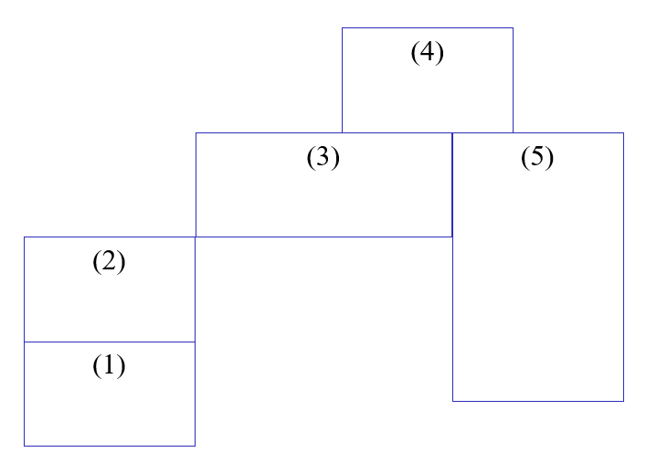
Le Sage page: 9 Figure 1.2 shows a hypothetical example of five regions as they would appear on a map. We wish to construct a 5 by 5 binary matrix W containing 25 elements taking values of 0 or 1 that captures the notion of “connectiveness” between the five entities depicted in the map congfiuration. We record in each row of the matrix W a set of contiguity relations associated with one of the five regions. For example the matrix element in row 1, column 2 would record the presence (represented by a 1) or absence (denoted by 0) of a contiguity relationship between regions 1 and 2. As another example, the row 3, column 4 element would reflect the presence or absence of contiguity between regions 3 and 4. Of course, a matrix constructed in such fashion must be symmetric | if regions 3 and 4 are contiguous, so are regions 4 and 3.
Rook contiguity: define
\[ w_{ij} = \begin{cases} 1, & \text{if regions } i \text{ and } j \text{ share a common side},\\ 0, & \text{otherwise}. \end{cases} \]
The diagonal is normally set to zero, \(w_{ii}=0\), because a region is not treated as its own neighbour.
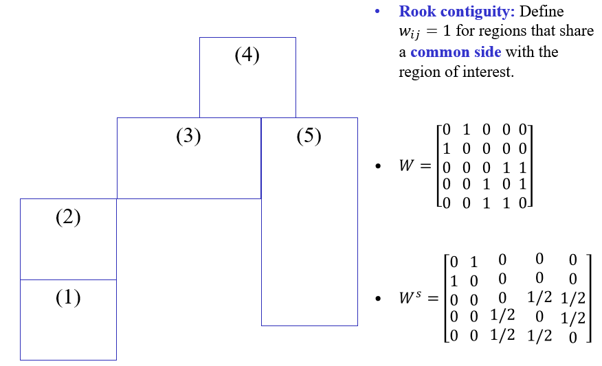
A transformation often used in applied work is to convert the matrix W to have row-sums of unity. This is referred to as a standardized first-order” contiguity matrix, which we denote as Ws
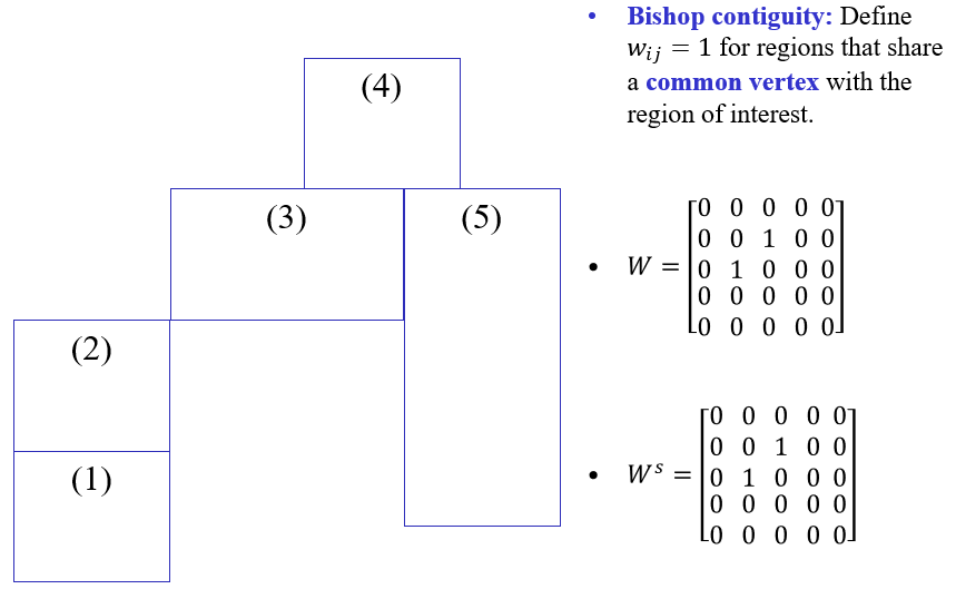
Bishop contiguity: define
\[ w_{ij} = \begin{cases} 1, & \text{if regions } i \text{ and } j \text{ share a common vertex only},\\ 0, & \text{otherwise}. \end{cases} \]
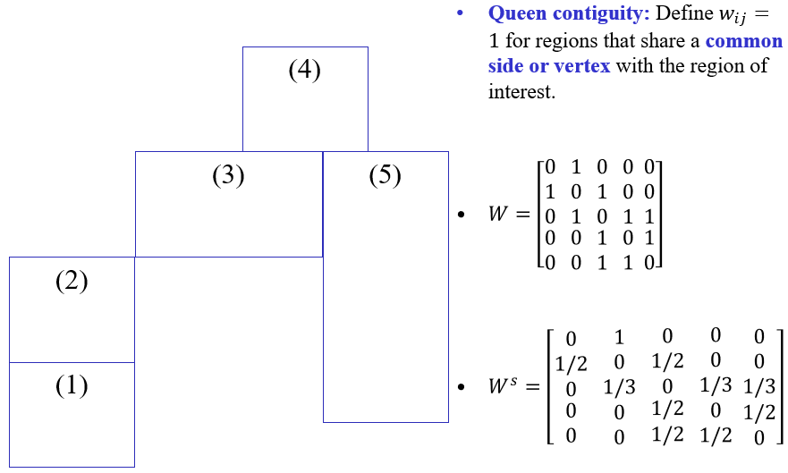
Queen contiguity: define
\[ w_{ij} = \begin{cases} 1, & \text{if regions } i \text{ and } j \text{ share a common side or vertex},\\ 0, & \text{otherwise}. \end{cases} \]
Believe it or not, there are even more ways one could proceed.
Difference between Queen and Rook
plot(st_geometry(columbus))
plot(queen_nb, coords, add=TRUE, col="red")
plot(rook_nb, coords, add=TRUE, col="blue")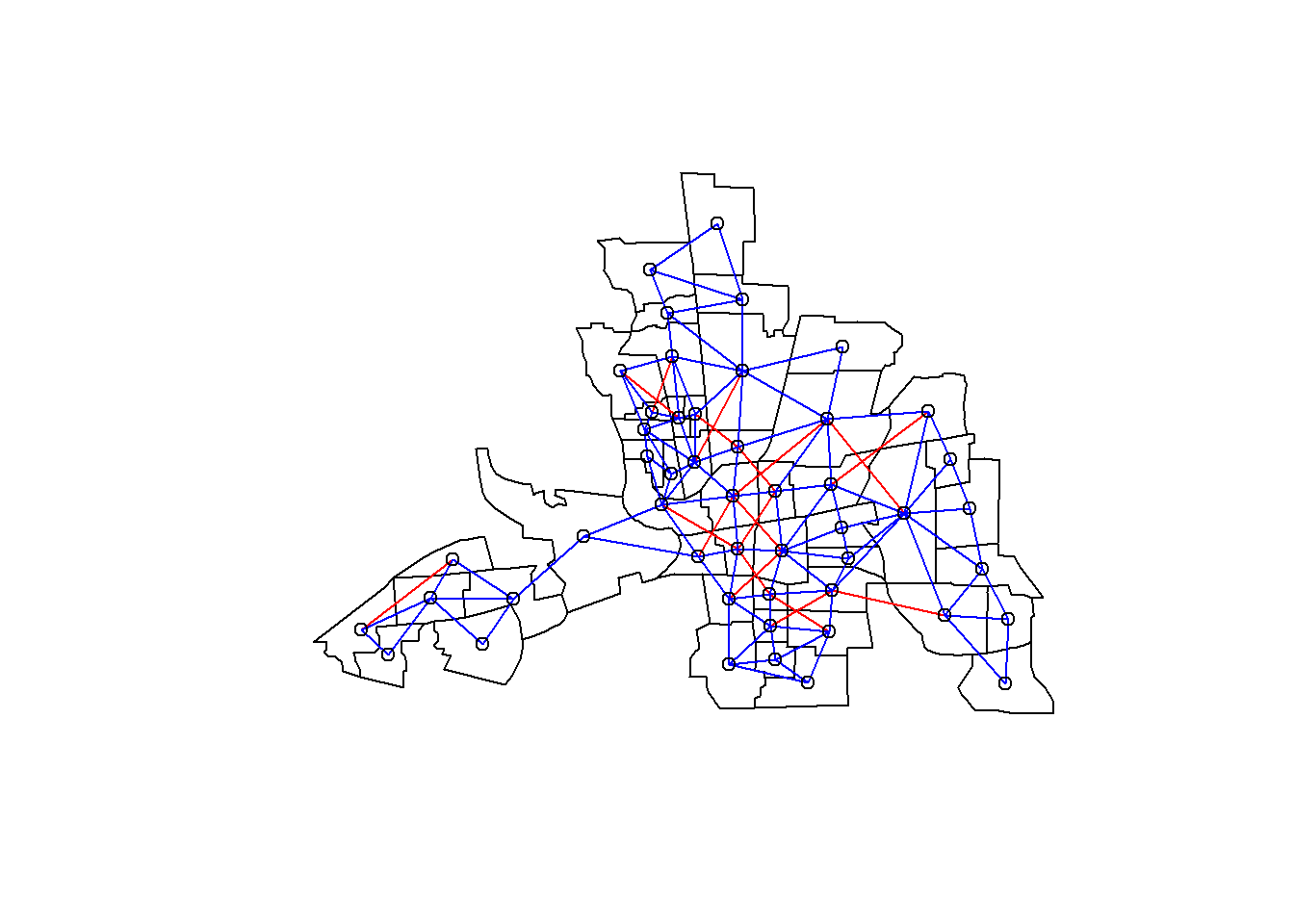
Neighbourhood relationships may also be defined by distance.
For each spatial unit \(i\), choose the \(k\) observations whose representative locations are closest to \(i\). (k)-nearest-neighbour neighbourhood
For the first-nearest-neighbour case,
\[ w_{ij} = \begin{cases} 1, & \text{if } d_{ij} = \displaystyle\min_{k \neq i} d_{ik}, \\[4pt] 0, & \text{otherwise}. \end{cases} \]
Two units (i) and (j) are neighbours if
\[ w_{ij} = \begin{cases} 1, & \text{if } d_{ij} < d^*, \\[4pt] 0, & \text{otherwise}. \end{cases} \]
where \(d_{ij}\) is the adopted distance measure and \(d^*\) is a chosen critical cut-off.
where distances are calculated from information on latitude and longitude of the centroid locations. Examples include straight-line distances, great circle distances, travel distances or times, and other spatial separation measures. Straight-line distances determine the shortest distance between any two point locations in a flat plane, treating longitude and latitude of a location as if they were equivalent to plane coordinates. In contrast, great circle distances determine distances between any two points on a spherical surface such as the earth as the length of the arc of the great circle between them (see Longley et al. 2001, pp. 86–92, for more details). In many applications the simple measures—straight-line distances and great circle distances—are not sufficiently accurate estimates of actual travel distances, and one is forced to resort to summing the actual lengths of travel routes, using a GISystem . This normally means summing the length of links in a network representation of a transportation system.
For observation (1), calculate pairwise centroid distances and identify the closest observation. The first-nearest-neighbour link is then entered in the neighbour structure.
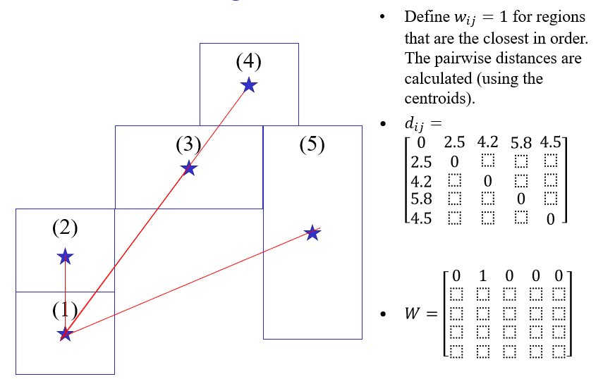
For observation (2), calculate pairwise centroid distances and identify the closest observation. The first-nearest-neighbour link is then entered in the neighbour structure.
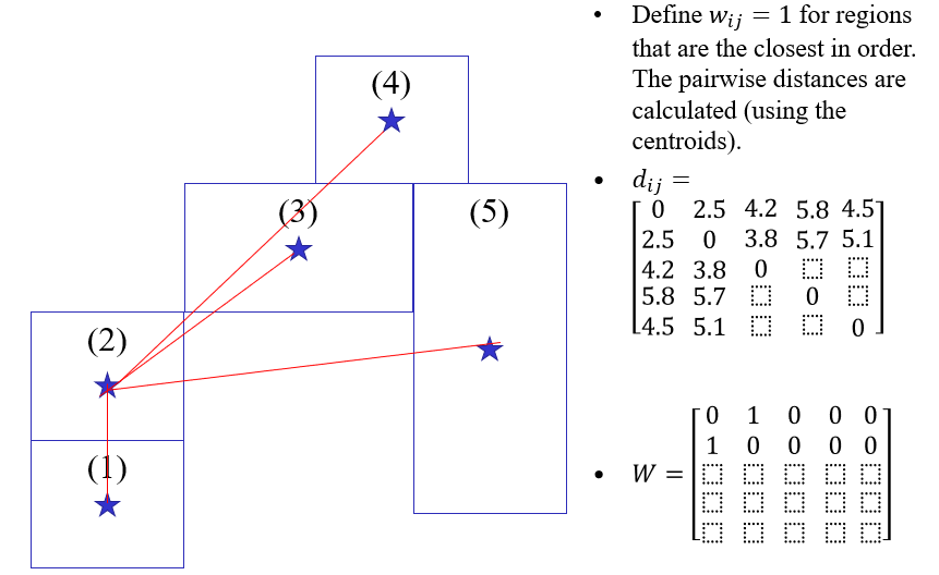
For observation (3), calculate pairwise centroid distances and identify the closest observation. The first-nearest-neighbour link is then entered in the neighbour structure.
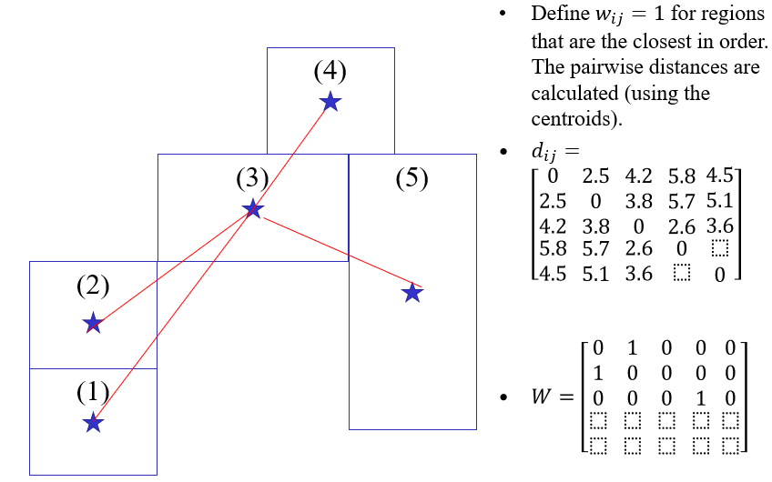
For observation (4), calculate pairwise centroid distances and identify the closest observation. The first-nearest-neighbour link is then entered in the neighbour structure.
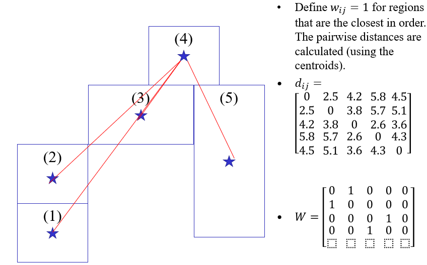
For observation (5), calculate pairwise centroid distances and identify the closest observation. The first-nearest-neighbour link is then entered in the neighbour structure.
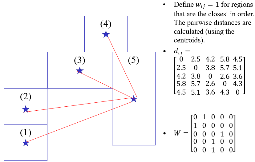
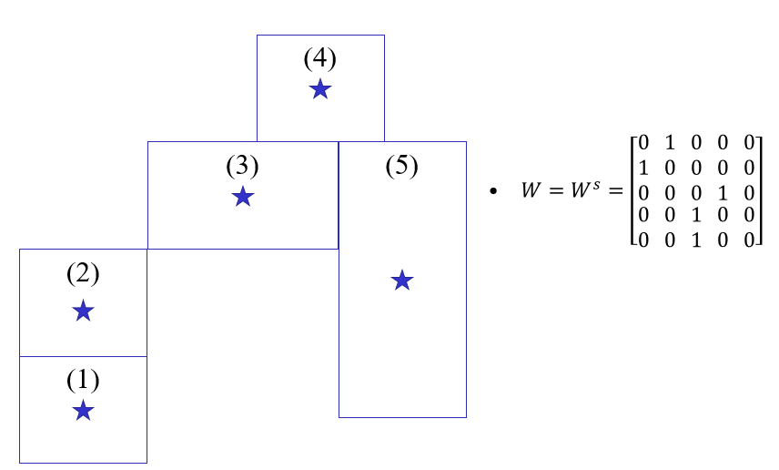
Combining the first-nearest-neighbour relationships for all five observations gives the complete first-nearest-neighbour graph.
library(sf)
library(spdep)

whoisthefirstnear=knearneigh(coords,k=1,longlat=TRUE)
knn1columbus=knn2nb(whoisthefirstnear)
plot(st_geometry(columbus))
plot(knn1columbus, coords, add=TRUE, col="blue")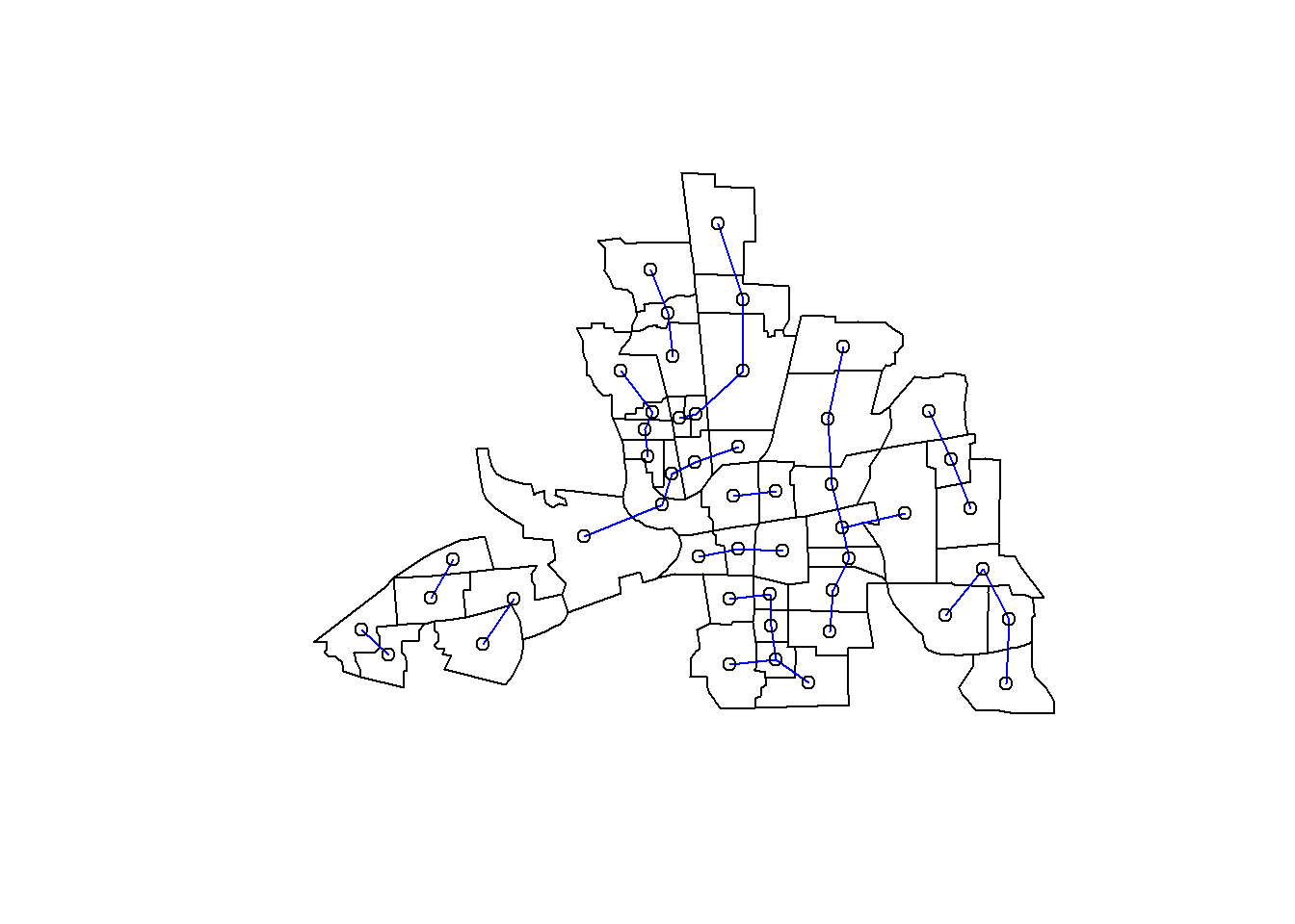
whois2near=knearneigh(coords,k=2,longlat=TRUE)
knn2columbus=knn2nb(whois2near)
plot(st_geometry(columbus))
plot(knn2columbus, coords, add=TRUE, col="blue")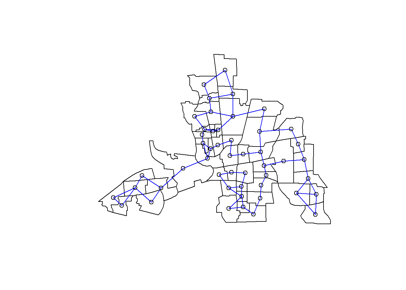
To define neighbours within a fixed distance, we need a threshold distance.
One way of selecting a threshold is:
distBetwNeigh1=nbdists(knn1columbus,coords,longlat=TRUE)
distBetwNeigh1=unlist(distBetwNeigh1)
distBetwNeigh1
[1] 63.98112 37.46759 57.90275 34.99180 50.68549 60.02289 41.50970 34.99180
[9] 53.16288 42.98225 13.85976 13.85976 15.87821 15.87821 36.74052 20.37838
[17] 42.32020 20.37838 21.89658 50.76316 67.50447 35.75701 42.32020 26.18731
[25] 34.14447 34.14447 25.62287 34.90927 32.08072 32.08072 35.72122 45.38893
[33] 25.62287 44.54357 28.40851 35.72122 32.67643 25.12110 29.91036 47.60799
[41] 45.38893 44.54357 25.12110 33.47541 37.48757 29.91036 51.94091 28.12354
[49] 32.04551For the Columbus example, the maximum first-nearest-neighbour distance is approximately
all.linkedTresh=max(distBetwNeigh1)
all.linkedTresh
[1] 67.50447dnbTresh1=dnearneigh(coords,0,68,longlat=TRUE)
summary(dnbTresh1)Neighbour list object:
Number of regions: 49
Number of nonzero links: 252
Percentage nonzero weights: 10.49563
Average number of links: 5.142857
2 disjoint connected subgraphs
Link number distribution:
1 2 3 4 5 6 7 8 9 10 11
4 8 6 2 5 8 6 2 6 1 1
4 least connected regions:
6 10 21 47 with 1 link
1 most connected region:
28 with 11 linksplot(st_geometry(columbus))
plot(dnbTresh1, coords, add=TRUE, col="blue")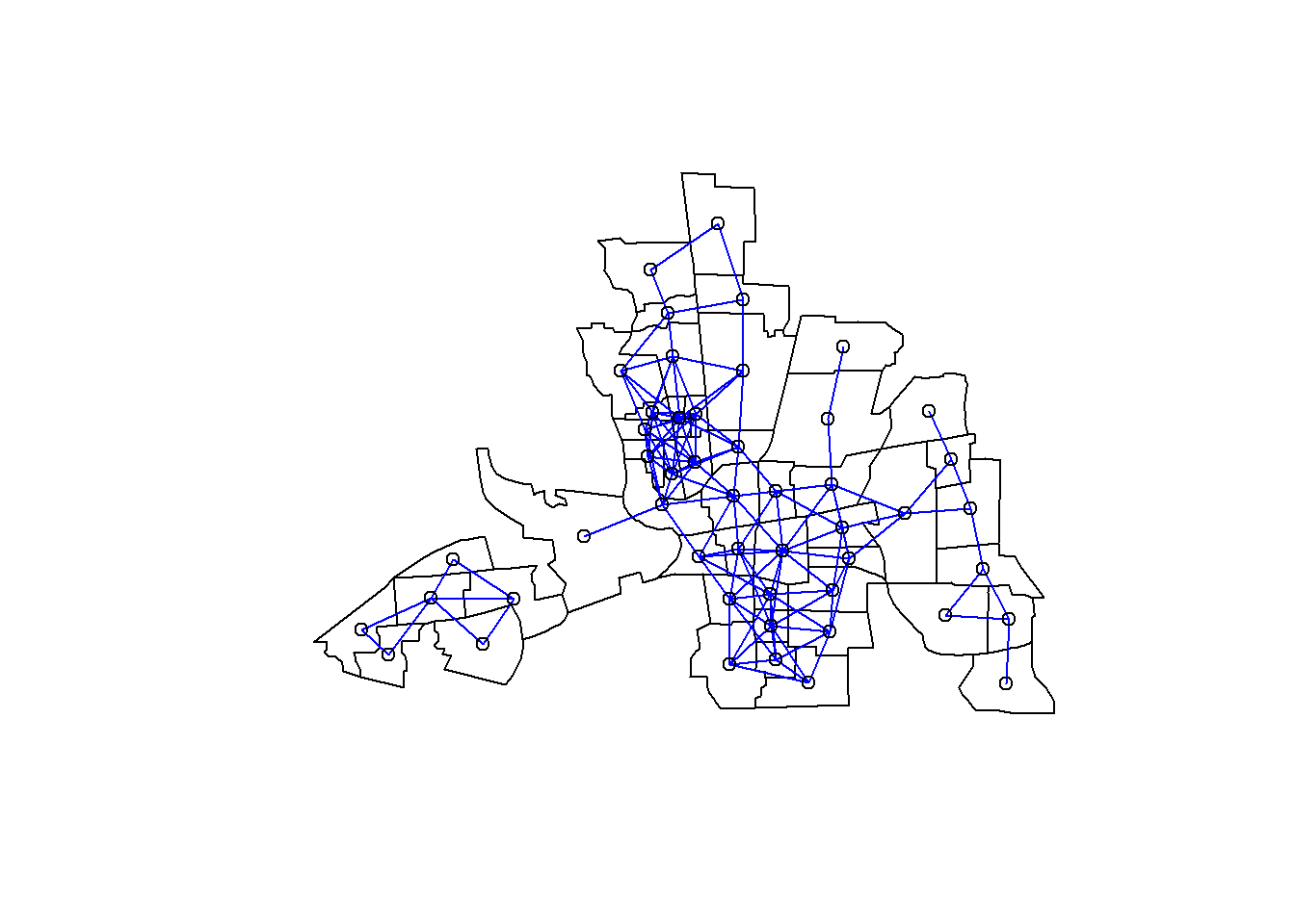
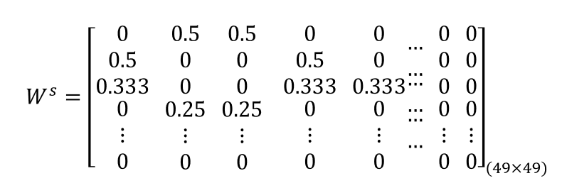
If you examine this neighbourhood list object a bit more closely you will see that, Polygon1 is neighbours with Poly2 and Poly3; Polygon2 is neighbours with Poly1 and Poly4; Polygon3 is neighbours with Poly1, Poly4 and Poly5 and so on:
dnbTresh1[1:3][[1]]
[1] 2 3
[[2]]
[1] 1 4
[[3]]
[1] 1 4 5In calculation of the weights that will be used to create the spatially lagged variables, only the neighbours values are going to be used. For example for the 1st Polygon, the values of neighbouring Poly2 and Poly3 will be used. Before doing this the nb values need to be standardized, so that the row
Here we will work with the Critical Cut-off nearest neighbours
dnbTresh1.listw=nb2listw(dnbTresh1,style="W",zero.policy=FALSE)
class(dnbTresh1.listw)
[1] "listw" "nb" dnbTresh1.listw$weights[1:5][[1]]
[1] 0.5 0.5
[[2]]
[1] 0.5 0.5
[[3]]
[1] 0.3333333 0.3333333 0.3333333
[[4]]
[1] 0.25 0.25 0.25 0.25
[[5]]
[1] 0.2 0.2 0.2 0.2 0.2In matrix format rather than a list:
listw2mat(dnbTresh1.listw)[1:5,1:5] 1 2 3 4 5
1 0.0000000 0.50 0.50 0.0000000 0.0000000
2 0.5000000 0.00 0.00 0.5000000 0.0000000
3 0.3333333 0.00 0.00 0.3333333 0.3333333
4 0.0000000 0.25 0.25 0.0000000 0.0000000
5 0.0000000 0.00 0.20 0.0000000 0.0000000Choosing a threshold of \(68\) therefore guarantees that every centroid has at least one neighbour. As you can see row sum of the \(W^s\) is always 1, we row-standardized the W matrix.
The level of spatial dependence (spatial autocorrelation) can be explored with:
Spatial autocorrelation tests are decision rules based on statistics such as Moran’s I and Geary’s c to assess the extent to which the observed spatial arrangement of data values departs from the null hypothesis that space does not matter. This hypothesis implies that near-by areas do not affect one another such that there is independence and spatial randomness. In contrast, under the alternative hypothesis of spatial autocorrelation (spatial association, spatial dependence), the interest renders on cases where large values are surrounded by other large values in near-by areas, or small values are surrounded by large values and vice versa. The former is referred to as positive spatial autocorrelation, and the latter as negative spatial autocorrelation. Positive spatial autocorrelation implies a spatial clustering of similar values, while negative spatial autocorrelation implies a checkerboard pattern of values
To simplify notation:
Moran’s \(I\) is a global measure: it provides one summary of spatial autocorrelation for the entire spatial pattern.
\[ I = \frac{Z'W^sZ}{Z'Z} \]
With row-standardised \(W^s\), this is closely related to the cross-product between the centred variable \(Z'=Y-\bar{Y}\) and its spatial lag \(W^sZ\).
Spatial autocorrelation is considered to be present when the spatial autocorrelation statistic computed for a particular pattern takes on a larger value, compared to what would be expected under the null hypothesis of no spatial association.
Under the randomisation null hypothesis, the expected value of Moran’s \(I\) is
\[ E(I)=-\frac{1}{n-1}. \]
Thus, under the null, Moran’s \(I\) is not centred exactly at zero for a finite sample. As \(n\) increases,
\[ E(I)\longrightarrow 0. \]
A standardised test statistic can be constructed as
\[ Z_I= \frac{I-E(I)} {\sqrt{\operatorname{Var}(I)}}. \]
The variance depends on the spatial weights and on the assumptions used for the reference distribution.
Ref: Fischer & Wang (2011), p. 25.
\[ \operatorname{Var}(I) = \frac{N S_4 - S_3 S_5} {(N-1)(N-2)(N-3)W^2} - [E(I)]^2 \]
where
\[ S_1 = \frac{1}{2} \sum_i \sum_j (w_{ij} - w_{ji})^2 \]
\[ S_2 = \sum_i \left( \sum_j w_{ij} - \sum_j w_{ji} \right)^2 \]
\[ S_3 = \frac{ N^{-1}\sum_i (x_i-\bar{x})^4 }{ \left[ N^{-1}\sum_i (x_i-\bar{x})^2 \right]^2 } \]
and
\[ S_4 = (N^2-3N+3)S_1 - NS_2 + 3W^2 \]
\[ S_5 = (N^2-N)S_1 - 2NS_2 + 6W^2 \]
Under spatial random process, the expected value of Moran’s I is given as follows. As you can see it is not centred around 0, it is a bit off to the negative side. And it depends on n, sample size. As n becomes larger and larger, Moran’s I gets closer to zero. The key question is the statistic that we obtained from the data, does it come from a spatial random process or not? In order to do the test we need the variance. As I mentioned earlier E(I)/Var(I) is comparable since the variance takes into account the different W values.
Two broad approaches are used to assess whether an observed Moran’s \(I\) departs significantly from the null hypothesis of no spatial autocorrelation:
Ref: lecture comparison example and linked video, around minute 22:25.
In principle, there are two main approaches to testing observed I -values for significant departure from the hypothesis of zero spatial autocorrelation. 1) Random permutation test 2) approximate sampling distribution of the I values.
For the Columbus CRIME variable, first centre the observations:
\[ z_i = y_i-\bar y. \]
The first part of the centred vector in the original analysis is:
columbus$CRIME - mean(columbus$CRIME) [1] -19.402844 -16.327070 -4.502043 -2.741064 15.602686 -9.062166
[7] -34.950555 3.297034 -4.612907 -1.127989 27.146624 21.576845
[13] 11.587305 21.937308 13.456663 19.709887 1.739950 8.833662
[19] 19.393141 -34.905027 4.945250 -1.423776 -15.080320 3.169047
[25] 26.170351 5.840918 17.665606 21.790961 25.621622 33.763220
[31] -17.451610 -15.983232 6.839339 -11.154796 4.046229 -20.823268
[37] 7.316252 18.582114 -16.027961 -18.887525 -16.223678 -18.636934
[43] 1.534788 -9.166561 -6.100336 -18.598291 -7.305963 -8.483558
[49] -12.587333The critical-cut-off neighbourhood is then represented through a row-standardised spatial weights matrix \(W^{(s)}\).
weightsmatrix_s = listw2mat(dnbTresh1.listw)
head(weightsmatrix_s)
1 2 3 4 5 6 7 8 9 10 11 12 13 14 15 16
1 0.0000000 0.50 0.50 0.0000000 0.0000000 0 0.00 0.00 0 0 0.0 0.0 0 0 0.0 0
2 0.5000000 0.00 0.00 0.5000000 0.0000000 0 0.00 0.00 0 0 0.0 0.0 0 0 0.0 0
3 0.3333333 0.00 0.00 0.3333333 0.3333333 0 0.00 0.00 0 0 0.0 0.0 0 0 0.0 0
4 0.0000000 0.25 0.25 0.0000000 0.0000000 0 0.25 0.25 0 0 0.0 0.0 0 0 0.0 0
5 0.0000000 0.00 0.20 0.0000000 0.0000000 0 0.00 0.20 0 0 0.2 0.2 0 0 0.2 0
6 0.0000000 0.00 0.00 0.0000000 0.0000000 0 0.00 0.00 1 0 0.0 0.0 0 0 0.0 0
17 18 19 20 21 22 23 24 25 26 27 28 29 30 31 32 33 34 35 36 37 38 39 40 41 42
1 0 0 0 0 0 0 0 0 0 0 0 0 0 0 0 0 0 0 0 0 0 0 0 0 0 0
2 0 0 0 0 0 0 0 0 0 0 0 0 0 0 0 0 0 0 0 0 0 0 0 0 0 0
3 0 0 0 0 0 0 0 0 0 0 0 0 0 0 0 0 0 0 0 0 0 0 0 0 0 0
4 0 0 0 0 0 0 0 0 0 0 0 0 0 0 0 0 0 0 0 0 0 0 0 0 0 0
5 0 0 0 0 0 0 0 0 0 0 0 0 0 0 0 0 0 0 0 0 0 0 0 0 0 0
6 0 0 0 0 0 0 0 0 0 0 0 0 0 0 0 0 0 0 0 0 0 0 0 0 0 0
43 44 45 46 47 48 49
1 0 0 0 0 0 0 0
2 0 0 0 0 0 0 0
3 0 0 0 0 0 0 0
4 0 0 0 0 0 0 0
5 0 0 0 0 0 0 0
6 0 0 0 0 0 0 0Using matrix notation with centred observations \(z\) and a row-standardised matrix \(W^{(s)}\),
\[ I= \frac{Z' W^sZ} {Z'Z}. \]
Y_s = columbus$CRIME - mean(columbus$CRIME)
lagY_s <- lag.listw(dnbTresh1.listw, Y_s)
moransI = t(Y_s)%*%weightsmatrix_s%*%Y_s/(t(Y_s)%*%Y_s)
moransI
[,1]
[1,] 0.5518257For the Columbus CRIME example in the lecture,
\[ I=0.5518257. \]
The reported randomisation test gives
\[ E(I)=-0.02083333,\qquad \operatorname{Var}(I)=0.01038068, \]
with a standard deviate of \(5.6206\) and a very small \(p\)-value.
moran.test(columbus$CRIME,dnbTresh1.listw)
    Moran I test under randomisation

data:  columbus$CRIME
weights: dnbTresh1.listw

Moran I statistic standard deviate = 5.6206, p-value = 9.514e-09
alternative hypothesis: greater
sample estimates:
Moran I statistic       Expectation          Variance
       0.55182569       -0.02083333        0.01038068
We need to do matrix calculations in order to calculate the Moran’s I statistic.
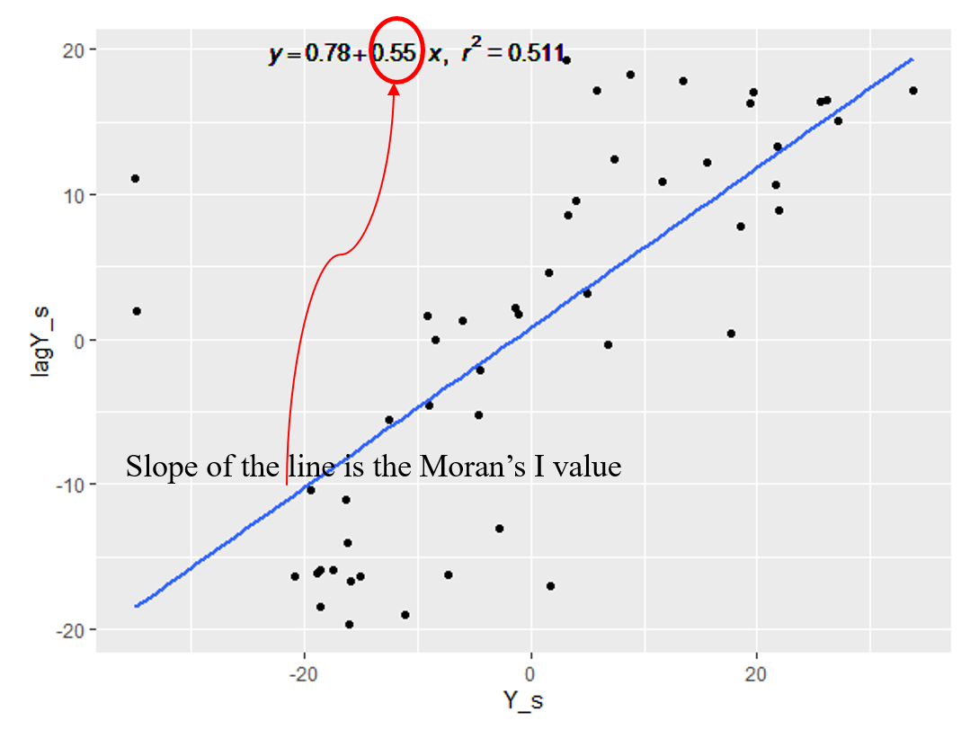
The Moran scatter plot places the centred or standardised variable on the horizontal axis and its spatial lag on the vertical axis:
\[ Z_i \quad \text{versus} \quad (WZ)_i. \]
When \(W\) and \(z\) are standardised consistently, the slope of the fitted line is Moran’s \(I\).
The plot therefore links the global statistic to the local behaviour of individual observations.
lm_eqn <- function(df, y, x){
    m <- lm(y ~ x, df);
    eq <- substitute(italic(y) == a + b %.% italic(x)*","~~italic(r)^2~"="~r2,
         list(a = format(unname(coef(m)[1]), digits = 2),
              b = format(unname(coef(m)[2]), digits = 2),
             r2 = format(summary(m)$r.squared, digits = 3)))
    as.character(as.expression(eq));
}

dataMoransI = data.frame(Y_s, lagY_s)

library(ggplot2)

ggplot(dataMoransI, aes(x = Y_s, y = lagY_s)) + geom_point() + geom_smooth(method = "lm", se=FALSE)+geom_text(x = -10, y = 20, label = lm_eqn(dataMoransI,lagY_s,Y_s), parse = TRUE)+geom_vline(xintercept=0, linetype="dashed", color = "red")+geom_hline(yintercept=0.78, linetype="dashed", color = "red")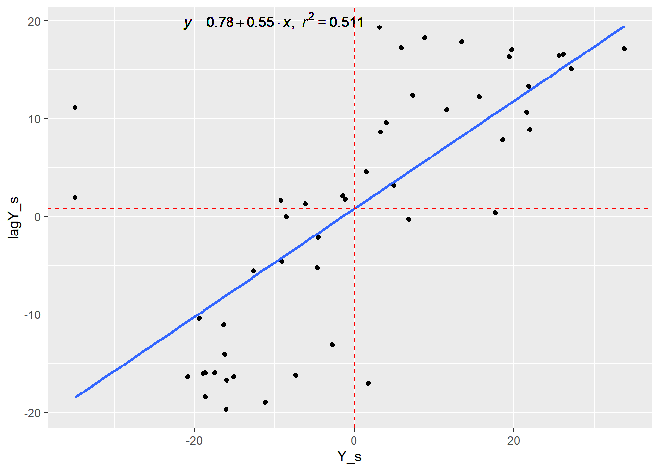
moran.plot(
  columbus$CRIME,
  dnbTresh1.listw,
  labels = row.names(columbus)
)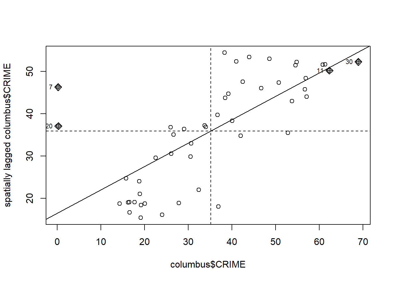
As you can see Moran’s I is the slope of the linear association between the attribute and its lagged values based on a weights matrix, should you use significance tests on this slope? NO. Why NOT? Need to be careful with outliers, since we all know the outliers influence the slope. What this plot helps us do is to move from global to local thinking.
we can also apply standard techniques for detecting observations with unusually strong influence on the slope. Specifically, moran.plot calls influence.measures on the linear model of lm ( wy ∼ y) providing the slope coefficient, where wy is the spatially lagged value of y .
The Moran scatter plot is partitioned into four quadrants:
| Quadrant | Observation | Neighbours | Interpretation |
|---|---|---|---|
| High–High | High | High | positive association / high-value cluster |
| Low–Low | Low | Low | positive association / low-value cluster |
| High–Low | High | Low | negative association / spatial outlier |
| Low–High | Low | High | negative association / spatial outlier |
The High–High and Low–Low quadrants represent positive spatial autocorrelation.
The High–Low and Low–High quadrants represent negative spatial autocorrelation.
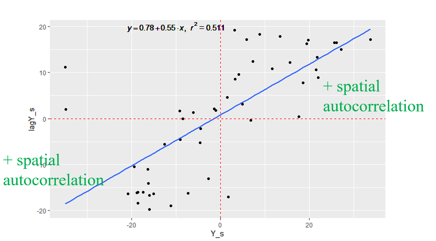
The plot is further partitioned into quadrants at the mean values of the variable and its lagged values: low–low, low–high, high–low, and high–high. We have the 4 quadrats of the scatter plot, where upper right and lower left indicate positive spatial autocorrelation indicating that locations are similar to their neighbours, whereas lower right and upper left show negative spatial autocorrelation which indicates the spatial outliers, locations are different from their neighbours.
Geary’s \(C\) focuses on squared differences between neighbouring observations:
\[ C= \frac{(n-1)}{2S_0} \frac{ \displaystyle\sum_{i=1}^{n}\sum_{j=1}^{n} w_{ij}(y_i-y_j)^2 }{ \displaystyle\sum_{i=1}^{n}(y_i-\bar y)^2 }. \]
where
\[ S_0=\sum_i\sum_j w_{ij}. \]
Interpretation is opposite in direction to Moran’s \(I\):
A non-parametric spatial correlogram is an alternative way of studying global spatial dependence.
Rather than beginning with one predefined weights matrix, it examines the association between pairs of observations as a function of their separation distance.
Conceptually,
\[ \operatorname{Cov}(z_i,z_j) = f(d_{ij})+\varepsilon_{ij}, \]
where
This allows us to ask how spatial association changes as distance increases.
Both Moran’s I and Geary’s C depend on weights matrices, coming from neighbourhood relationships. Most people would find this description arbitrary. In fact there are tons of different neighbourhood descriptions one can make. It might be worthwhile investigating other ways of measuring spatial autocorrelation.
Here we see the values of Moran’s I for ten successive lag orders of contiguous neighbours. The Figure shows the output plot from spdep package with sp.correlogram () function, and suggests that second-order neighbours are also positively autocorrelated. The horizontal line is the expected Moran’s I under no spatial autocorrelation.
Local Indicators of Spatial Association (LISA) were introduced by Anselin (1995) to decompose global spatial autocorrelation into contributions from individual observations.
A common form of the local Moran statistic for area \(i\) is
\[ I_i = \frac{z_i}{m_2} \sum_j w_{ij}z_j, \]
where
\[ z_i=y_i-\bar y, \qquad m_2=\frac{1}{n}\sum_i z_i^2. \]
The summation runs over the neighbourhood of area \(i\).
The collection of local Moran statistics is related to the global Moran statistic: their sum is proportional to global Moran’s \(I\).
With the advent of large data sets characteristic of GISystems , it has become clear that the need to assess spatial autocorrelation globally may be of only marginal interest. During the past two decades, a number of statistics, called local statistics, have been developed. These provide for each observation of a variable an indication of the extent of significant spatial clustering of similar values around that observation. Hence, they are well suited to identify the existence of hot spots (local clusters of high values) or cold spots (local clusters of low values), and are appropriate to identify distances beyond which no discernible association exists. Local indicators of spatial association (LISA) statistics were derived by Anselin (1995), in his paper of Local Indicators of Spatial Association—LISA published in Geographical Analysis in 1995. An initial evaluation of the properties of a LISA statistic is carried out for the local Moran, which is applied in a study of the spatial pattern of conflict for African countries and in a number of Monte Carlo simulations. HE suggests that a local indicator of spatial association (LISA) is any statistic that satisfies the following two requirements a) the LISA for each observation gives an indication of the extent of significant spatial clustering of similar values around that observation; b. the sum of LISAs for all observations is proportional to a global indicator of spatial association. The local Moran statistic is defined as follows: where denotes the neighbourhood set of area (can be formalized by means of a spatial weights or contiguity matrix) , and the summation in runs only over those areas belonging to , denotes the average of these neighbouring observations. The LISA statistic, Ii serve two purposes. On the one hand, they may be viewed as indicators of local pockets of non-stationarity, or hot spots. On the other hand, they may be used to assess the influence of individual locations (observations) on the magnitude of the corresponding global spatial autocorrelation statistic, Moran’s I With the advent of large data sets characteristic of GISystems , it has become clear that the need to assess spatial autocorrelation globally may be of only marginal interest. During the past two decades, a number of statistics, called local statistics, have been developed. These provide for each observation of a variable an indication of the extent of significant spatial clustering of similar values around that observation. Hence, they are well suited to identify the existence of hot spots (local clusters of high values) or cold spots (local clusters of low values), and are appropriate to identify distances beyond which no discernible association exists. Local indicators of spatial association (LISA) statistics were derived by Anselin (1995), in his paper of Local Indicators of Spatial Association—LISA published in Geographical Analysis in 1995. An initial evaluation of the properties of a LISA statistic is carried out for the local Moran, which is applied in a study of the spatial pattern of conflict for African countries and in a number of Monte Carlo simulations. HE suggests that a local indicator of spatial association (LISA) is any statistic that satisfies the following two requirements a) the LISA for each observation gives an indication of the extent of significant spatial clustering of similar values around that observation; b. the sum of LISAs for all observations is proportional to a global indicator of spatial association. The local Moran statistic is defined as follows: where 𝐽_𝑖 denotes the neighbourhood set of area 𝑖 (can be formalized by means of a spatial weights or contiguity matrix) , and the summation in 𝑗 runs only over those areas belonging to 𝐽_𝑖 , 𝑧 ̅ denotes the average of these neighbouring observations. The LISA statistic, Ii serve two purposes. On the one hand, they may be viewed as indicators of local pockets of non-stationarity, or hot spots. On the other hand, they may be used to assess the influence of individual locations (observations) on the magnitude of the corresponding global spatial autocorrelation statistic, Moran’s I
Local spatial clusters—often called hot spots or cold spots—may be identified as locations, or sets of contiguous locations, for which a LISA statistic is significant.
The null hypothesis is no local spatial association.
Because the exact distribution of a generic LISA statistic can be difficult to obtain, a common alternative is a conditional randomisation / permutation procedure that produces empirical pseudo-\(p\)-values.
A test for significant local spatial association may be based on the moments, although the exact distribution of such a statistic is still unknown ( Anselin 1995, p. 99). Alternatively, a conditional random permutation test can be used to yield so-called pseudo significance levels . (for example, as in Hubert 1987). The randomization is conditional in the sense that the value Yi at a location i is held fixed (that is, not used in the permutation) and the remaining values are randomly permuted over the locations in the data set. For each of these resampled data sets, the value of Li can be computed. The resulting empirical distribution function provides the basis for a statement about the extremeness (or lack of extremeness) of the observed statistic, relative to (and conditional on) the values computed under the null hypothesis (the randomly permuted values). In practice, this is straightforward to implement, since for each location only as many values as there are in the neighborhood set need to be resampled. Note that this same approach can also easily be applied to the Gi and GT statistics.
localmoranstatistics = localmoran(Y_s,dnbTresh1.listw)
head(localmoranstatistics)
Ii E.Ii Var.Ii Z.Ii Pr(z != E(Ii))
1 0.73681849 -0.0285985420 0.666144891 0.9378077 0.34834327
2 0.65915397 -0.0202502140 0.475741297 0.9850149 0.32461676
3 0.03579329 -0.0015396867 0.024041007 0.2407777 0.80972741
4 0.13113818 -0.0005707572 0.006541757 1.6284260 0.10343458
5 0.69380337 -0.0184931910 0.162742823 1.7656716 0.07745096
6 0.15242670 -0.0062384562 0.303777355 0.2878749 0.77344247columbus$localmoran = localmoranstatistics[,1]Plot of the Local Moran Statistics
tm_shape(columbus) + tm_polygons(style="quantile", col = "localmoran") +
     tm_legend(outside = TRUE, text.size = .8)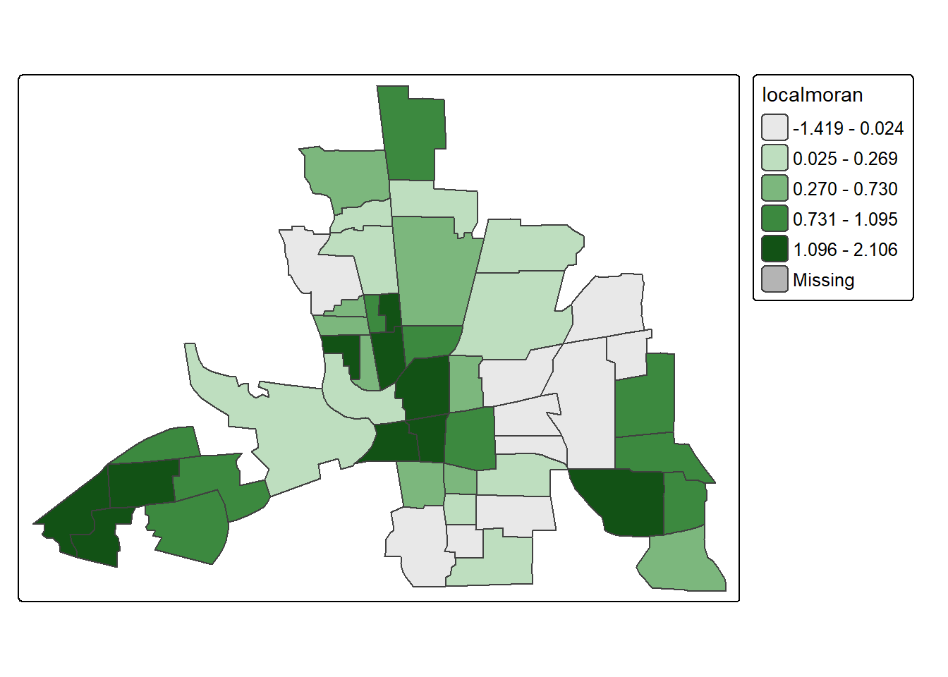
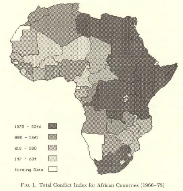
Measures of spatial association, such as Moran’s I, have been applied to quantitative indices for various types of conflicts and cooperation between nation-states in Africa, such as those contained in the COPDAB data base (Azar 1980). The spatial pattern of the index for total conflict is illustrated in the quartile map in Figure 1, with the darkest shade corresponding to the highest quartile [for details on the data sources, see Anselin and O’Loughlin (1992)]. The suggestion of spatial clustering of similar values that follows from a visual inspection of this map is confirmed by a strong positive and significant Moran’s I of 0.417, with an associated standard normal z-value of 4.35 (p < 0.001), These statistics are computed for a row-standardized spatial weights matrix based on first-order contiguity (common border), given the importance of borders in the study of international conflict. Allcomputationswere carried out with the SpaceStat softwarefor spatial data analysis
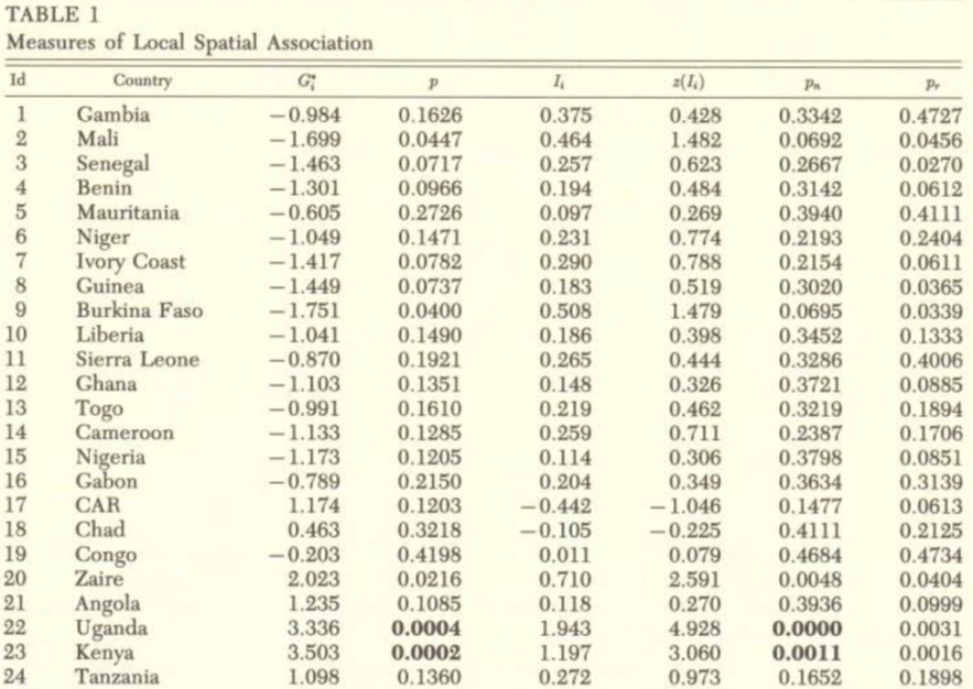
Using the same row-standardized weights matrix as for the global measures given earlier, the results for the indicators of local spatial association are reported in the third and fifth columns of Table 1, for each of the forty-two countries in the example. The standardized z-value for Ii , computed by subtracting the expected value (13) and dividing by the standard deviation [the square root of (14)], is listed in the sixth column. Two indications of significance are given, one based on an approximation by the normal distribution, Pn (in the seventh column of Table 1) and one derived from conditional randomization, using a sample of 10,000 permutations, Pr (in the last column of Table 1). Given this conservative procedure, the normal approximation for both the Gi and the Ii show the same four countries to exhibit local spatial clustering (with the significance levels in bold type in Table 1). They are Uganda (22), Kenya (23), Sudan (41), and Egypt (42), which themselves form a cluster in the northeast of Africa, part of the so-called Shatterbelt . Shatter belt is a concept in geopolitics according to which on the political map are recognized and analyzed strategically positioned and oriented regions that are deeply internally divided and encompassed in the competition between the great powers in the geostrategic areas and spheres
In R, local Moran statistics can be calculated with spdep::localmoran():
localmoranstatistics <- spdep::localmoran(
  Y_s,
  dnbTresh1.listw
)

localmoranstatistics
Ii E.Ii Var.Ii Z.Ii Pr(z != E(Ii))
1 0.736818491 -2.859854e-02 0.6661448908 0.93780765 0.3483432685
2 0.659153968 -2.025021e-02 0.4757412970 0.98501488 0.3246167634
3 0.035793288 -1.539687e-03 0.0240410072 0.24077770 0.8097274126
4 0.131138176 -5.707572e-04 0.0065417568 1.62842603 0.1034345818
5 0.693803371 -1.849319e-02 0.1627428232 1.76567158 0.0774509642
6 0.152426700 -6.238456e-03 0.3037773549 0.28787494 0.7734424674
7 -1.418605235 -9.279429e-02 0.7547857820 -1.52605345 0.1269965546
8 0.103319296 -8.257717e-04 0.0050383143 1.46722284 0.1423154446
9 0.088187389 -1.616451e-03 0.0386977724 0.45651171 0.6480220495
10 -0.007156422 -9.665465e-05 0.0047356202 -0.10258928 0.9182889508
11 1.489116910 -5.598153e-02 0.2387512105 3.16215652 0.0015660536
12 0.834073870 -3.536625e-02 0.1351553596 2.36495586 0.0180322198
13 0.459183376 -1.019948e-02 0.0526252173 2.04611609 0.0407449499
14 0.708918984 -3.655778e-02 0.1591203691 1.86883613 0.0616456170
15 0.875366588 -1.375586e-02 0.0828431006 3.08911022 0.0020075694
16 1.223927852 -2.951083e-02 0.1293875235 3.48463177 0.0004928147
17 -0.108094629 -2.299782e-04 0.0035956407 -1.79883361 0.0720450046
18 0.587470453 -5.927816e-03 0.0266215244 3.63688706 0.0002759529
19 1.151223098 -2.856995e-02 0.1694747499 2.86584918 0.0041589234
20 -0.247951607 -9.255269e-02 0.7530211176 -0.17907889 0.8578757561
21 0.057144088 -1.857760e-03 0.0908611332 0.19573863 0.8448147484
22 -0.010918574 -1.539914e-04 0.0011236363 -0.32113253 0.7481099581
23 0.900849470 -1.727564e-02 0.2654944353 1.78186236 0.0747716792
24 0.222445111 -7.629051e-04 0.0046550365 3.27150994 0.0010697483
25 1.576737186 -5.202741e-02 0.2570965315 3.21225647 0.0013169675
26 0.366611808 -2.591644e-03 0.0188644701 2.68808779 0.0071862501
27 0.023496701 -2.370665e-02 0.1689066665 0.11485488 0.9085601515
28 1.054294593 -3.607164e-02 0.1219320577 3.12257905 0.0017927395
29 1.534813119 -4.986851e-02 0.2893304273 2.94608293 0.0032182610
30 2.106237710 -8.659660e-02 0.5772443881 2.88619691 0.0038992811
31 1.017447516 -2.313578e-02 0.5419314656 1.41352881 0.1575002960
32 0.975052651 -1.940628e-02 0.2975917603 1.82295690 0.0683099184
33 -0.008281905 -3.553378e-03 0.0258399512 -0.02941576 0.9765330041
34 0.771608734 -9.452275e-03 0.1464202875 2.04119422 0.0412315257
35 0.140766915 -1.243695e-03 0.0090650426 1.49154332 0.1358189064
36 1.243242522 -3.293904e-02 0.2856021104 2.38798590 0.0169409917
37 0.330451865 -4.066216e-03 0.0247289081 2.12724311 0.0333998888
38 0.529422011 -2.623031e-02 0.1153931242 1.63573582 0.1018948896
39 1.151957408 -1.951505e-02 0.4588139896 1.72947288 0.0837244959
40 1.109043195 -2.709962e-02 0.6322045881 1.42890746 0.1530308318
41 0.831677994 -1.999456e-02 0.3064288938 1.53853646 0.1239175009
42 1.086553172 -2.638530e-02 0.6159922141 1.41802388 0.1561837935
43 0.025506418 -1.789410e-04 0.0008082627 0.90346090 0.3662813328
44 -0.055325820 -6.383017e-03 0.0462851033 -0.22749310 0.8200403375
45 -0.028304126 -2.826966e-03 0.0252748048 -0.16025335 0.8726815086
46 1.249537703 -2.627600e-02 0.6135092567 1.62883353 0.1033482644
47 0.432196383 -4.054787e-03 0.1978789359 0.98070146 0.3267399841
48 0.002170906 -5.467253e-03 0.0396811746 0.03834391 0.9694134795
49 0.254910325 -1.203595e-02 0.1363680392 0.72288227 0.4697522160
attr(,"call")
spdep::localmoran(x = Y_s, listw = dnbTresh1.listw)
attr(,"class")
[1] "localmoran" "matrix" "array"
attr(,"quadr")
mean median pysal
1 Low-Low Low-Low Low-Low
2 Low-Low Low-Low Low-Low
3 Low-Low Low-Low Low-Low
4 Low-Low Low-Low Low-Low
5 High-High High-High High-High
6 Low-Low Low-Low Low-Low
7 Low-High Low-High Low-High
8 High-High High-High High-High
9 Low-Low Low-Low Low-Low
10 Low-High Low-Low Low-High
11 High-High High-High High-High
12 High-High High-High High-High
13 High-High High-High High-High
14 High-High High-High High-High
15 High-High High-High High-High
16 High-High High-High High-High
17 High-Low High-Low High-Low
18 High-High High-High High-High
19 High-High High-High High-High
20 Low-High Low-High Low-High
21 High-High High-High High-High
22 Low-High Low-High Low-High
23 Low-Low Low-Low Low-Low
24 High-High High-High High-High
25 High-High High-High High-High
26 High-High High-High High-High
27 High-Low High-Low High-High
28 High-High High-High High-High
29 High-High High-High High-High
30 High-High High-High High-High
31 Low-Low Low-Low Low-Low
32 Low-Low Low-Low Low-Low
33 High-Low High-Low High-Low
34 Low-Low Low-Low Low-Low
35 High-High High-High High-High
36 Low-Low Low-Low Low-Low
37 High-High High-High High-High
38 High-High High-High High-High
39 Low-Low Low-Low Low-Low
40 Low-Low Low-Low Low-Low
41 Low-Low Low-Low Low-Low
42 Low-Low Low-Low Low-Low
43 High-High High-High High-High
44 Low-High Low-Low Low-High
45 Low-High Low-Low Low-High
46 Low-Low Low-Low Low-Low
47 Low-Low Low-Low Low-Low
48 Low-Low Low-Low Low-Low
49 Low-Low Low-Low Low-LowThe output provides a local statistic for every spatial unit, together with quantities used for inference.