STA5092Z EDA Lecture 7-8

Tidy Datasets

“Happy families are all alike; every unhappy family is unhappy in its own way.” L.Tolstoy - Anna Karenina

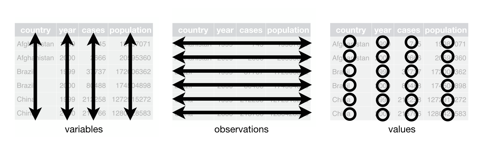
Like families, tidy datasets are all alike but every messy dataset is messy in its own way. A dataset is messy or tidy depending on how rows, columns and tables are matched up with observations, variables and types. In tidy data:

Each variable must have its own column.
Each observation must have its own row.
Each value must have its own cell.

Ref: https://r4ds.had.co.nz/tidy-data.html

Why do we need tidy data?

Tidy datasets are all alike but every messy dataset is messy in its own way.

This clearly states that:

There is uniformity
R works in vectorised nature.

Are we ever going to work with untidy datasets? Answer is all the time… What type of issues can we have with untidy datasets?

One variable might be spread across multiple columns.
One observation might be spread across multiple rows.

library(tidyverse)

treatmentdata <- tibble(
  person = c("JS", "JD", "MJ"),
  treatmenta = as.numeric(c(NaN, 16,3)),
  treatmentb = c(12,11,1)
  )
treatmentdata |> kableExtra::kable()

Table 1: Treatment a-b values for patients

person	treatmenta	treatmentb
JS	NaN	12
JD	16	11
MJ	3	1

Table 2 shows the same data as Table 1, but the rows and columns have been transposed. The data is the same, but the layout is different.

Table 2: Treatment a-b values for patients - Observations in columns

person	JS	JD	MJ
treatmenta	NA	16	3
treatmentb	12	11	1

Reorganised dataset

Table 3 is the tidy version of Table 1. Each row represents an observation, the result of one treatment on one person, and each column is a variable. We will see how we can obtain this tidy dataset in R.

Table 3: Treatment a-b values for patients - Observations in columns

person	treatment	cases
JS	treatmenta	NaN
JS	treatmentb	12
JD	treatmenta	16
JD	treatmentb	11
MJ	treatmenta	3
MJ	treatmentb	1

Tidying messy datasets

Most common problems with messy datasets are

Column headers are values, not variable names.
One variable might be spread across multiple columns.
A single observational unit might be scattered across multiple rows.
Multiple variables are stored in one column.
Variables are stored in both rows and columns.
Multiple types of observational units are stored in the same table.

To fix these problems, you’ll need the two most important functions in tidyr: pivot_longer() and pivot_wider()

`pivot_longer()` table4a

pivot_longer() makes datasets longer by increasing the number of rows and decreasing the number of columns.

Column headers are values, not variable names.
One variable might be spread across multiple columns.

table4a

# A tibble: 3 × 3
  country     `1999` `2000`
  <chr>        <dbl>  <dbl>
1 Afghanistan    745   2666
2 Brazil       37737  80488
3 China       212258 213766

tidy4a <- table4a |>
  pivot_longer(c('1999', '2000'), 
               names_to = "year", 
               values_to = "cases")

`pivot_longer()` table4b

table4b

# A tibble: 3 × 3
  country         `1999`     `2000`
  <chr>            <dbl>      <dbl>
1 Afghanistan   19987071   20595360
2 Brazil       172006362  174504898
3 China       1272915272 1280428583

tidy4b <- table4b |>   
  pivot_longer(c('1999', '2000'),
               names_to = "year",
               values_to = "population")

`pivot_longer()` tidy4a and tidy4b

tidy4a

# A tibble: 6 × 3
  country     year   cases
  <chr>       <chr>  <dbl>
1 Afghanistan 1999     745
2 Afghanistan 2000    2666
3 Brazil      1999   37737
4 Brazil      2000   80488
5 China       1999  212258
6 China       2000  213766

tidy4b

# A tibble: 6 × 3
  country     year  population
  <chr>       <chr>      <dbl>
1 Afghanistan 1999    19987071
2 Afghanistan 2000    20595360
3 Brazil      1999   172006362
4 Brazil      2000   174504898
5 China       1999  1272915272
6 China       2000  1280428583

`full_join()`

full_join(tidy4a, tidy4b)

Joining with `by = join_by(country, year)`

# A tibble: 6 × 4
  country     year   cases population
  <chr>       <chr>  <dbl>      <dbl>
1 Afghanistan 1999     745   19987071
2 Afghanistan 2000    2666   20595360
3 Brazil      1999   37737  172006362
4 Brazil      2000   80488  174504898
5 China       1999  212258 1272915272
6 China       2000  213766 1280428583

`pivot_wider()` table2

A single observational unit might be scattered across multiple rows

table2

# A tibble: 12 × 4
   country      year type            count
   <chr>       <dbl> <chr>           <dbl>
 1 Afghanistan  1999 cases             745
 2 Afghanistan  1999 population   19987071
 3 Afghanistan  2000 cases            2666
 4 Afghanistan  2000 population   20595360
 5 Brazil       1999 cases           37737
 6 Brazil       1999 population  172006362
 7 Brazil       2000 cases           80488
 8 Brazil       2000 population  174504898
 9 China        1999 cases          212258
10 China        1999 population 1272915272
11 China        2000 cases          213766
12 China        2000 population 1280428583

`pivot_wider()`

We need to tell R from which column the variable names are coming from.
We also need to tell R from which column the variable values are coming from.
For more examples and explanation see vignette("pivot")

table2 |> 
  pivot_wider(names_from = type, 
              values_from = count)

# A tibble: 6 × 4
  country      year  cases population
  <chr>       <dbl>  <dbl>      <dbl>
1 Afghanistan  1999    745   19987071
2 Afghanistan  2000   2666   20595360
3 Brazil       1999  37737  172006362
4 Brazil       2000  80488  174504898
5 China        1999 212258 1272915272
6 China        2000 213766 1280428583

`separate()`

Multiple variables are stored in one column.

table3

# A tibble: 6 × 3
  country      year rate             
  <chr>       <dbl> <chr>            
1 Afghanistan  1999 745/19987071     
2 Afghanistan  2000 2666/20595360    
3 Brazil       1999 37737/172006362  
4 Brazil       2000 80488/174504898  
5 China        1999 212258/1272915272
6 China        2000 213766/1280428583

table3 |>
  separate(rate, 
           into = c("cases", "population"), 
           sep = "/",
           convert=TRUE)

# A tibble: 6 × 4
  country      year  cases population
  <chr>       <dbl>  <int>      <int>
1 Afghanistan  1999    745   19987071
2 Afghanistan  2000   2666   20595360
3 Brazil       1999  37737  172006362
4 Brazil       2000  80488  174504898
5 China        1999 212258 1272915272
6 China        2000 213766 1280428583

Combining Datasets

Mutating joins: left, right, inner, full

Mini example 1

a <- tibble(x1 = c("A", "B", "C"),
                  x2 = c(1, 2, 3)
                 )
b <- tibble(x1 = c("A", "B", "D"),
                  x3 = c("T", "F", "T")
                 )

`left_join()`

Join all rows from the second dataset that match exactly to the first dataset.

leftJoin <- left_join(a, b, by = "x1")

`right_join()`

Join all rows from the first dataset that match exactly to the second dataset.

rightJoin <- right_join(a, b, by = "x1")

Try with by x2 and see what happens?

`inner_join()`

Join the two datasets by retaining only the exact matching rows in both datasets.

innerJoin <- inner_join(a, b, by = "x1")

`full_join()`

Join the two datasets by retaining all rows in both datasets.

fullJoin <- full_join(a, b, by = "x1")

Filtering Joins

`semi_join()` and `anti_join()`

Retain all rows in the 1st dataset that have a match in the 2nd

semiJoin <- semi_join(a, b, by = "x1")

Retain only the rows in the 1st dataset that DO NOT have a match in the 2nd

antiJoin <- anti_join(a, b, by = "x1")

Set operations: intersect, union, setdiff; Binding operations: bind rows, columns

Mini example 2

y <- tibble(x1 = c("A", "B", "C"),
        x2 = c(1, 2, 3)
        )

z <- tibble(x1 = c("B", "C", "D"),
        x2 = c(2, 3, 4)
        )

`intersect()`

Rows that appear in both y AND z (exact match) for all variables

inters <- intersect(y, z)

`union()`

Rows that appear in EITHER y OR z for all variables

union <- union(y, z)

What could be the potential error here?

`setdiff()`

Rows that appear in both y BUT NOT z for all variables

setdifferent <- setdiff(y, z)

`bind_rows()`

Append both datasets along the rows without ANY MATCHING, datasets can have different variables, different number of rows.

bindrows <- bind_rows(y, z)

When would this be the most useful? What could be improved?

`bind_rows()` with id

Append both datasets along the rows without ANY MATCHING, and include which dataset the observation belongs to

bindrows <- dplyr::bind_rows(y, z, .id = "id")

`bind_rows()` with id as a year variable

Append both datasets along the rows without ANY MATCHING, and include which dataset the observation belongs to

bindrows <- bind_rows("1990" = y, "2001" = z, .id = "year")

Check the class for year variable!

`bind_cols()`

Append both datasets along columns without ANY MATCHING (except row index, need to have exact number of observations in both datasets)

bindcolumns <- bind_cols(y, z)

New names:
• `x1` -> `x1...1`
• `x2` -> `x2...2`
• `x1` -> `x1...3`
• `x2` -> `x2...4`

What would happen if the datasets have different number of observations?

One final note

Some older functions don’t work with tibbles. If you encounter one of these functions, use as.data.frame() to turn a tibble back to a data.frame:

tibbledata <- tibble(x1 = c(1,2,3))
class(tibbledata)

[1] "tbl_df"     "tbl"        "data.frame"

dataframe <- as.data.frame(tibbledata)
class(dataframe)

[1] "data.frame"

References

Once you learn the dplyr grammar there are a few additional benefits . dplyr can work with other data frame “backends”” such as SQL databases. There is an SQL interface for relational databases via the DBI package . dplyr can be integrated with the data.table package for large fast tables

Managing Data Frames with Package

Key TIDYR verbs

gather(): Gather (or “melt”) wide data into long format
spread(): Spread (or “cast”) long data into wide format.
separate(): Separate (i.e. split) one column into multiple columns.
unite(): Unite (i.e. combine) multiple columns into one.

STA5092Z EDA Lecture 7-8

Tidy Datasets

Why do we need tidy data?

Reorganised dataset

Tidying messy datasets

pivot_longer() table4a

pivot_longer() table4b

pivot_longer() tidy4a and tidy4b

full_join()

pivot_wider() table2

pivot_wider()

separate()

Combining Datasets

Mutating joins: left, right, inner, full

Mini example 1

left_join()

right_join()

inner_join()

full_join()

Filtering Joins

semi_join() and anti_join()

Set operations: intersect, union, setdiff; Binding operations: bind rows, columns

Mini example 2

intersect()

union()

setdiff()

bind_rows()

bind_rows() with id

bind_rows() with id as a year variable

bind_cols()

One final note

References

Managing Data Frames with Package

Key TIDYR verbs

`pivot_longer()` table4a

`pivot_longer()` table4b

`pivot_longer()` tidy4a and tidy4b

`full_join()`

`pivot_wider()` table2

`pivot_wider()`

`separate()`

`left_join()`

`right_join()`

`inner_join()`

`full_join()`

`semi_join()` and `anti_join()`

`intersect()`

`union()`

`setdiff()`

`bind_rows()`

`bind_rows()` with id

`bind_rows()` with id as a year variable

`bind_cols()`