Applied Spatial Data Analysis

Chapter 3 - Spatial Lattice Data I

Dr. Şebnem Er

Department of Statistical Sciences, University of Cape Town

1 Modelling Lattice Data

Exploratory spatial data analysis is often a preliminary step to more formal modelling approaches. In spatial lattice data, the goal is often to explain variation in a variable observed for each areal unit using other variables recorded for those same areal units.

In this lecture, the focus moves from exploratory spatial dependence to spatial regression models in a simple cross-sectional setting.

The key question is:

what happens to regression modelling when observations are spatially dependent?

Exploratory spatial data analysis is often a preliminary step to more formal modelling approaches that seek to establish relationships between the observations of a variable and the observations of other variables, recorded for each areal unit. The focus in this chapter is on spatial regression models in a simple crosssectional setting

1.1 Spatial Regression Models

Our starting point is the ordinary linear regression model. For each lattice observation or areal unit \(i=1,\ldots,N\), let

\[ y_i = \sum_f^F x_{if}\beta_f + \varepsilon_i. \]

Equivalently, in matrix form,

\[ y = X\beta + \varepsilon, \]

where \(y\) is an \((N\times 1)\) vector of observations, \(X\) is an \((N\times F)\) matrix of explanatory variables, \(\beta\) is the vector of regression coefficients, and \(\varepsilon\) is the error vector.

In the classical regression specification:

\[ E(\varepsilon_i)=0, \]

\[ \operatorname{Var}(\varepsilon_i)=\sigma^2, \]

and, for \(i\neq j\),

\[ \operatorname{Cov}(\varepsilon_i,\varepsilon_j)=0. \]

Thus the errors are assumed to be independent and identically distributed, with constant variance and no correlation across observations.

The assumption of independent observations greatly simplifies the model. However, for areal data this is often unrealistic because neighbouring areas may influence one another or may share omitted spatially structured variables.

If the regressors, residuals or the dependent variable are spatially dependent, the model suffers from a misspecification problem and the results of the model are biased or inconsistent.

1.1.1 Columbus dataset

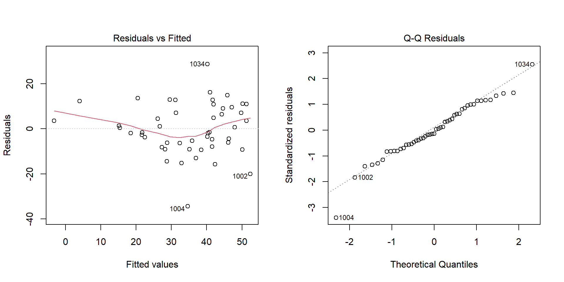
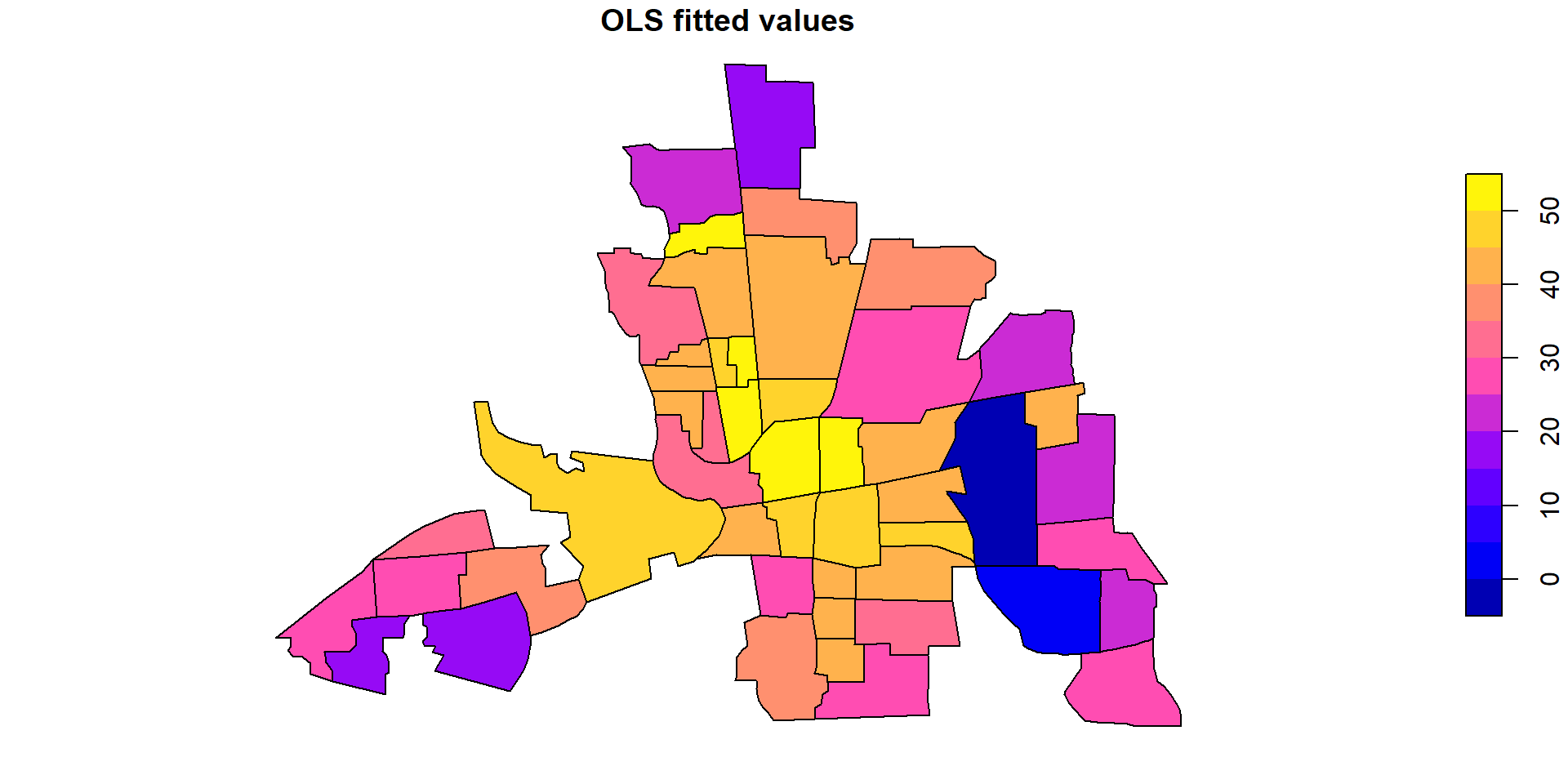
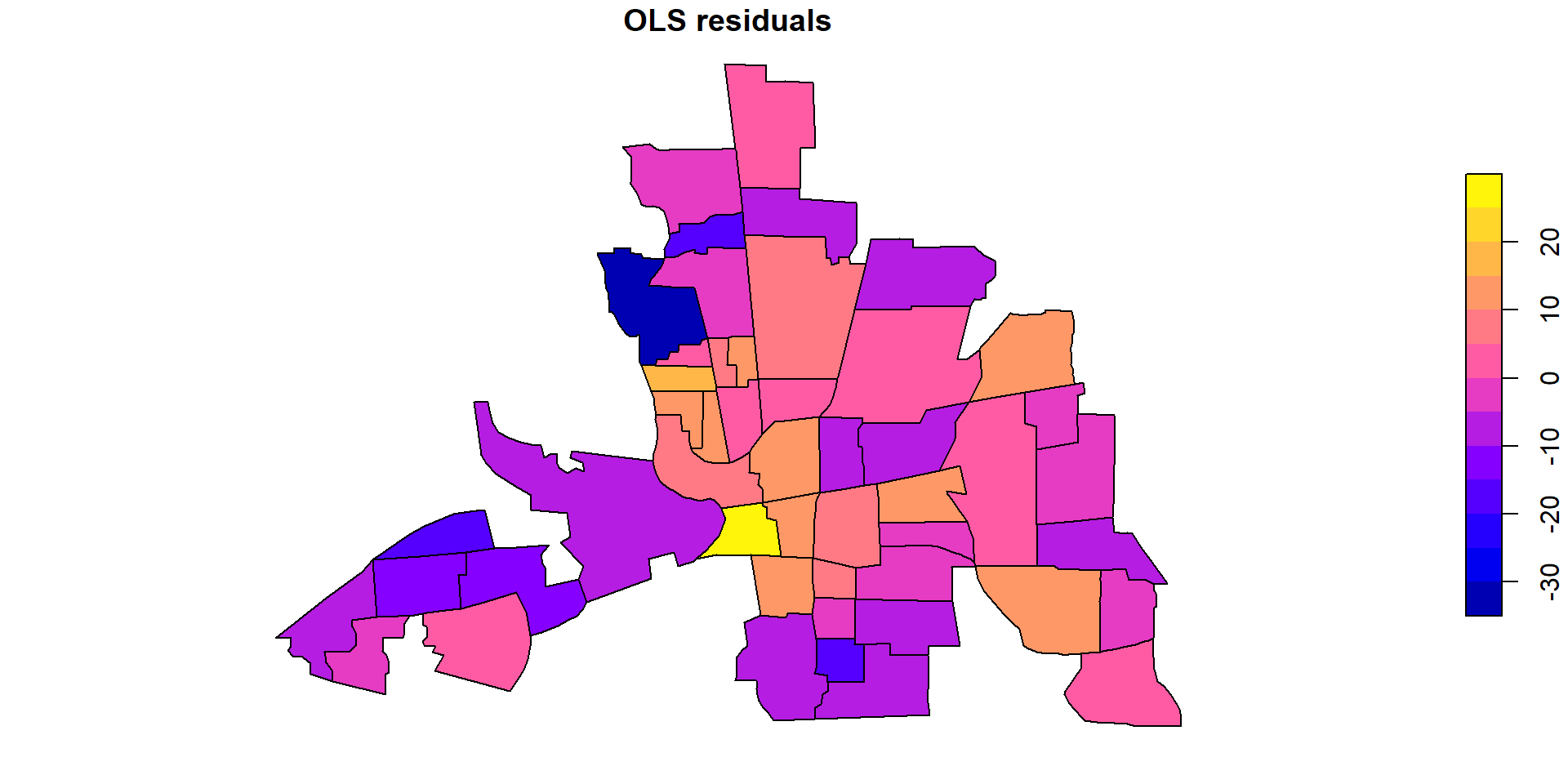
We begin with the Columbus data and model crime as a function of income and housing value using OLS:

\[ \text{CRIME}_i = \beta_0+ \beta_1\text{INC}_i+ \beta_2\text{HOVAL}_i+ \varepsilon_i. \]

library(spData)
library(spdep)
library(spatialreg)

data("columbus", package = "spData")

OLScolumbus <- lm(CRIME ~ INC + HOVAL, data = columbus)
summary(OLScolumbus)

Call:
lm(formula = CRIME ~ INC + HOVAL, data = columbus)

Residuals:
    Min      1Q  Median      3Q     Max 
-34.418  -6.388  -1.580   9.052  28.649 

Coefficients:
            Estimate Std. Error t value Pr(>|t|)    
(Intercept)  68.6190     4.7355  14.490  < 2e-16 ***
INC          -1.5973     0.3341  -4.780 1.83e-05 ***
HOVAL        -0.2739     0.1032  -2.654   0.0109 *  
---
Signif. codes:  0 '***' 0.001 '**' 0.01 '*' 0.05 '.' 0.1 ' ' 1

Residual standard error: 11.43 on 46 degrees of freedom
Multiple R-squared:  0.5524,    Adjusted R-squared:  0.5329 
F-statistic: 28.39 on 2 and 46 DF,  p-value: 9.341e-09

All estimated coefficients are strongly significant. The fit is reasonable (0.552 in terms of rsquared ) We are going to obviously look at the residuals.

1.1.2 OLS – Residuals vs Fitted Plot & Q-Q Plot

The first diagnostic step is to inspect standard OLS residual plots.

• The residuals versus fitted plot checks patterns in the residuals, non-linearity, and changing variance.
• The Q-Q plot checks whether residuals are approximately normally distributed.

par(mfrow = c(1, 2))
plot(OLScolumbus, which = 1)
plot(OLScolumbus, which = 2)

par(mfrow = c(1, 1))

1.1.3 Predicted and Residual Maps

Predicted values and residuals can be mapped to see whether model performance varies spatially.

If areas with similar residuals cluster together, this suggests that the OLS model has left spatial structure unexplained.

A typical mapping workflow is:

example(columbus)

colmbs> columbus <- st_read(system.file("shapes/columbus.gpkg", package="spData")[1], quiet=TRUE)

colmbs> col.gal.nb <- read.gal(system.file("weights/columbus.gal", package="spData")[1])

columbus$ols_fitted <- fitted(OLScolumbus)
columbus$ols_resid  <- residuals(OLScolumbus)

plot(columbus["ols_fitted"], main = "OLS fitted values")

plot(columbus["ols_resid"],  main = "OLS residuals")

This map does suggest that similarly colored areas tend to be in similar locations, which could indicate positive spatial autocorrelation (a Moran’s I test for residual spatial autocorrelation is positive and highly significant). Also, it indicates a tendency to overpredict (negative residuals) in the outlying areas and a tendency to underpredict (positive residuals) in the core, suggesting the possible presence of spatial heterogeneity in the form of spatial regimes.

1.1.4 Moran’s I Test for Residual Spatial Autocorrelation

The next step is to test for residual spatial autocorrelation using Moran’s \(I\) applied to the OLS model residuals.

In R:

coords <- st_coordinates(st_centroid(st_geometry(columbus)))
dnbTresh1=dnearneigh(coords,0,68,longlat=TRUE)
dnbTresh1.listw=nb2listw(dnbTresh1,style="W",zero.policy=FALSE)

col.moran <- lm.morantest(
  OLScolumbus,
  dnbTresh1.listw
)

col.moran

    Global Moran I for regression residuals

data:  
model: lm(formula = CRIME ~ INC + HOVAL, data = columbus)
weights: dnbTresh1.listw

Moran I statistic standard deviate = 3.0562, p-value = 0.001121
alternative hypothesis: greater
sample estimates:
Observed Moran I      Expectation         Variance 
     0.266348450     -0.032344498      0.009551988 

The LM test for spatial autocorrelation in the error term has a slightly lower significance than that indicated by a traditional Moran test, although this is a general statement we can make. Why not simply apply Moran’s I test on the residuals? (Ref: anselinintrospatregres.pdf page 11) Also: Roger Bivand’s book page: 281: Since the Moran test is intended to detect spatial autocorrelation, we can try to fit a model taking this into account.We should not, however, forget that the misspecifications detected by Moran’s I can have a range of causes (see Sect. 9.4). It is also the case that if the fitted model exhibits multi-collinearity, the results of the test may be affected because of the numerical consequences of the model matrix not being of full rank for the expectation and variance of the statistic.

1.2 Spatial Models

Spatial regression models introduce spatial dependence explicitly into the regression framework.

The main specifications in this lecture are:

• spatial lag / spatial autoregressive models;
• spatial error models;
• combined spatial lag and spatial error models;
• diagnostic tests that help choose between them.

1.2.1 General Spatial Autoregressive (Lag) Models

A general spatial autoregressive model for cross-sectional lattice data can be written as a SARAR or spatial lag-error model:

\[ y = \rho W_1^s y + Z\beta + u, \]

\[ u = \lambda W_2^s u + \varepsilon, \]

with

\[ \varepsilon \sim N(0,\sigma^2 I). \]

Here:

• \(y\) is the dependent variable;
• \(Z\) is the matrix of explanatory variables which can include the lagged explanatory variables as well, \(Z=[X,W_3^sX]\);
• \(W_1\) is the spatial weights matrix for the lagged dependent variable;
• \(W_2\) is the spatial weights matrix for the error process;
• \(\rho\) is the spatial autoregressive lag coefficient \(| \rho|<1\);
• \(\lambda\) is the spatial autoregressive error coefficient \(|\lambda|<1\);
• \(u\) is the spatially structured disturbance;
• \(\varepsilon\) is the innovation error term.

The model can also be written as:

\[ (I-\rho W_1)y = X\beta + u, \]

and

\[ (I-\lambda W_2)u = \varepsilon. \]

Special models are obtained by imposing restrictions such as \(\rho=0\), \(\lambda=0\), or removing \(X\beta\).

Where \(\rho\) represents a regression parameter to be estimated and epsilon denotes the stochastic disturbance in the relationship. The parameter rho would reflect the spatial dependence inherent in our sample data, measuring the average influence of neighboring or contiguous observations on observations in the vector y . If we posit spatial dependence between the individual observations in the data sample y , some part of the total variation in y across the spatial sample would be explained by each observation’s dependence on its neighbors. The parameter would reflect this in the typical sense of regression. In addition, we could calculate the proportion of the total variation in y that is explained by spatial dependence.

1.2.2 Special Forms of Spatial Autoregressive (Lag) Models

From the general form, we obtain several special cases.

1.2.2.1 First-order spatial autoregressive model

If there are no explanatory variables and no spatial error process:

\[ y = \rho W_1^sy + \varepsilon. \]

This model explains variation in \(y\) through neighbouring values of \(y\) and \(\epsilon \sim N(0,\sigma^2 I_N)\).

1.2.2.2 Spatial lag model / SAR model

If explanatory variables are included but the error term is not spatially autocorrelated:

\[ y = \rho W_1^sy + X\beta + \varepsilon. \]

\(\epsilon \sim N(0,\sigma^2 I_N)\)

1.2.2.3 Spatial error model

If spatial dependence enters through the disturbances:

\[ y = X\beta + u, \]

\[ u = \lambda W^s_2u + \varepsilon. \]

1.2.2.4 Spatial lag-error model / SARAR model

If both processes are present:

\[ y = \rho W_1^sy + X\beta + u, \]

\[ u = \lambda W_2^su + \varepsilon. \]

Moran’s \(I\) for the OLS residuals may indicate spatial dependence, but by itself it does not tell us whether the dependence should be modelled as a spatial lag, a spatial error process, or both.

From the general form we can derive special models by imposing restrictions. First order spatial autoregressive model attempts to explain variation in y as a linear combination of contiguous or neighboring units with no other explanatory variables S patial error dependence : spatial correlation in the error term Morans I for the OLS residuals indicate a spatial dependence but which way around is it? Is it a spatial lag, error or both? Hence, it has become convenient to distinguish between spatial lag and spatial error model specifications. These models require the application of special estimation procedures. Why not OLS?

1.3 Problems with OLS

OLS is problematic when the true model contains spatial dependence.

The consequences depend on where the spatial dependence appears:

• if the dependent variable is spatially lagged, the spatial lag \(Wy\) is endogenous;
• if the error term is spatially autocorrelated, the OLS coefficients may be inefficient and the usual standard errors are invalid;
• if the spatial process is misspecified, coefficient estimates and inference can be biased or inconsistent.

This motivates special estimation procedures such as maximum likelihood and instrumental variables.

1.3.1 First Order Spatial Lag Model with OLS

Consider the simplest first-order spatial lag model without explanatory variables:

\[ y = \rho W^sy + \varepsilon. \]

The SAR specification uses neighbouring values of \(y\) to account for spatial dependence.

The spatially lagged variable is

\[ W^sy, \]

which is usually interpreted as a weighted average of neighbouring values when \(W\) is row-standardised.

If \(y\) is mean standardised, the model focuses on deviations from the overall mean.

For the simple model

\[ y=\rho Wy+\varepsilon, \]

OLS treats \(Wy\) as an explanatory variable. The OLS estimator of \(\rho\) is

\[ \hat\rho_{OLS} = \left[(Wy)'(Wy)\right]^{-1}(Wy)'y. \]

Equivalently,

\[ \hat\rho_{OLS} = \frac{y'W'y}{y'W'Wy}. \]

If \(W\) is symmetric, this is often written as

\[ \hat\rho_{OLS} = \frac{y'Wy}{y'W'Wy}. \]

The problem is that \(Wy\) is not exogenous. Because \(y\) itself is generated through a spatial feedback process, \(Wy\) is correlated with the error structure.

Let us take the simple form with no X variables. Y variable is mean standardized

1.3.2 First Order Spatial Autoregressive Model with OLS

For OLS to be consistent, the explanatory variable must be asymptotically uncorrelated with the error term. In the simple spatial lag model this requires a condition of the form

\[ \frac{1}{N}(Wy)'\varepsilon \longrightarrow 0. \]

However, in the spatial case this condition generally fails. Since

\[ y = (I-\rho W)^{-1}\varepsilon, \]

we have

\[ Wy = W(I-\rho W)^{-1}\varepsilon. \]

Therefore,

\[ (Wy)'\varepsilon = \varepsilon'\left[(I-\rho W)^{-1}\right]'W'\varepsilon. \]

This is a quadratic form in the error terms, and it is not generally equal to zero.

Consequently, the OLS estimator is biased and inconsistent for the spatial lag parameter.

Refer to the hand written notes here.

1.4 Maximum Likelihood Estimation

Because OLS is inappropriate for models with spatial dependence, maximum likelihood estimation becomes a natural alternative.

Maximum likelihood estimates the model parameters by choosing the values that make the observed vector \(y\) most likely under the assumed spatial data-generating process.

The likelihood must account for two important transformations:

1. the transformation from \(y\) to the spatially filtered response \((I-\rho W)y\);
2. the transformation from the spatially structured disturbance \(u\) to the innovation \((I-\lambda W)u\).

These transformations introduce Jacobian terms into the likelihood.

1.4.1 Spatial Lag + Error Model

The spatial lag-error model can be written as

\[ y = \rho W_1^s y + Z\beta + u, \]

\[ u = \lambda W_2^s u + \varepsilon. \]

Equivalently,

\[ (I-\rho W_1^s)y = Z\beta + u, \]

and

\[ (I-\lambda W_2^s)u = \varepsilon. \]

Solving for the disturbance gives

\[ u=(I-\rho W_1^s)y-Z\beta. \]

The innovation term is therefore

\[ \varepsilon = (I-\lambda W_2^s) \left[(I-\rho W_1^s)y-Z\beta\right]. \]

1.4.2 The Likelihood Function and the Jacobian for the General Model

For the general spatial lag-error model, the likelihood is built from the transformation between \(y\) and the normally distributed innovation term.

Define

\[ B(\rho)=I-\rho W_1^s, \]

and

\[ A(\lambda)=I-\lambda W_2^s. \]

Then

\[ u=B(\rho)y-Z\beta, \]

and

\[ \varepsilon=A(\lambda)u = A(\lambda)\{B(\rho)y-Z\beta\}. \]

The change of variables from \(y\) to \(\varepsilon\) contributes the Jacobian terms

\[ |B(\rho)| = |I-\rho W_1^s| \]

and

\[ |A(\lambda)| = |I-\lambda W_2^s|. \]

The log-likelihood for the general model contains the normal density component plus the spatial Jacobian terms.

Using the notation from the lecture, one form is

\[ \ell = -\frac{n}{2}\ln(\pi) - \frac{1}{2}\ln(|\Omega|) + \ln\left(|I-\rho W_1^s|\right) + \ln\left(|I-\lambda W_2^s|\right) - \frac{1}{2}v'v. \]

Here \(v\) is the transformed, standardised residual vector implied by the spatial model.

The maximum likelihood estimator chooses the values of the parameters, including \(\rho\), \(\lambda\), \(\beta\), and variance parameters, that maximise this log-likelihood.

Ref: Anselin, p. 63; see also Anselin et al. (1996).

We can either use, Maximum Likelihood estimation Instrumental Variables We will look at MLE. Y variable is mean standardized

1.4.3 Calculation of the Jacobian Term

There are several ways to calculate the Jacobian term, especially the log determinant

\[ \log|I-\rho W|. \]

1.4.3.1 Exact approaches

• eigenvalues, Ord (1975), used in R with method = "eigen";
• LU decomposition, method = "LU";
• Cholesky decomposition, method = "Matrix";
• sparse Cholesky decomposition, method = "spam".

1.4.3.2 Approximate approaches

• Chebyshev approximation, Pace and LeSage (2004), method = "Chebyshev";
• Monte Carlo approximation, Barry and Pace (1999), method = "MC".

Exact methods should agree up to numerical precision. Approximate methods should give similar values when the approximation is sufficiently accurate.

The default method of method="full" uses eigenvalues, and can thus also set the lower and upper bounds for the line search for \(\lambda\) accurately (as \(\left[\frac{1}{\min_i(\zeta_i)},\frac{1}{\max_i(\zeta_i)}\right]\)), but is not feasible for large \(n\). It should also be noted that although eigenvalues are computed for intrinsically asymmetric spatial weights matrices, their imaginary parts are discarded, so that even for method="full", the consequences of using such asymmetric weights matrices are unknown.

Alternative approaches involve finding the log determinant of a Cholesky decomposition of the sparse matrix

\[ (I - \lambda W) \]

directly. Here it is not possible to pre-compute eigenvalues, so one log determinant is computed for each value of \(\lambda\) used, but the number needed is in general not excessive, and much larger \(n\) become feasible on ordinary computers.

A number of different sparse matrix approaches have been tried, with the use of Matrix and method="Matrix" the one suggested currently. All of the sparse matrix approaches to computing the Jacobian require that matrix \(W\) be symmetric or at least similar to symmetric, thus providing for weights with "W" and "S" styles based on symmetric neighbour lists and symmetric general spatial weights, such as inverse distance.

Matrices that are similar to symmetric have the same eigenvalues, so that the eigenvalues of symmetric

\[ W^* = D^{1/2} B D^{1/2} \]

and row-standardised

\[ W = DB \]

are the same, for symmetric binary or general weights matrix \(B\), and \(D\) a diagonal matrix of inverse row sums of \(B\),

\[ d_{ii} = \frac{1}{\sum_{j=1}^{n} b_{ij}} \]

(Ord, 1975, p. 125).

1.5 Hypothesis Tests Based on the ML Principles

Maximum likelihood estimation naturally leads to several hypothesis-testing frameworks.

1.5.1 Wald test

Tests restrictions using the estimated parameter and its estimated variance.

1.5.2 Likelihood ratio test

Compares the maximised likelihoods of a restricted and an unrestricted model.

1.5.3 Lagrange multiplier test

Evaluates whether adding a spatial parameter would improve the model, using estimates from the restricted model, usually OLS.

1.6 Example: Columbus Dataset

The Columbus data frame has 49 rows and 22 columns.

The main variables used here are:

• CRIME: residential burglaries and vehicle thefts per thousand households in the neighbourhood;
• INC: household income;
• HOVAL: housing value.

library(spData)
data("columbus", package = "spData")

nrow(columbus)
ncol(columbus)
names(columbus)
summary(columbus[, c("CRIME", "INC", "HOVAL")])

1.7 OLS

1.7.1 Model 0: OLS with INC and HOVAL

Model 0 is the OLS model with income and housing value:

\[ \text{CRIME}_i = \beta_0+ \beta_1\text{INC}_i+ \beta_2\text{HOVAL}_i+ \varepsilon_i. \]

In R:

OLScolumbus <- lm(
  CRIME ~ INC + HOVAL,
  data = columbus
)

summary(OLScolumbus)

All estimated coefficients are strongly significant. The fit is reasonable (0.552 in terms of rsquared ) We are going to obviously look at the residuals.

1.7.1.1 Moran’s I Test for Residual Spatial Autocorrelation

The OLS residuals are tested for spatial autocorrelation.

col.moran <- lm.morantest(
  OLScolumbus,
  dnbTresh1.listw
)

summary(col.moran)

The LM test for spatial autocorrelation in the error term has a slightly lower significance than that indicated by a traditional Moran test, although this is a general statement we can make. Why not simply apply Moran’s I test on the residuals? (Ref: anselinintrospatregres.pdf page 11) Also: Roger Bivand’s book page: 281: Since the Moran test is intended to detect spatial autocorrelation, we can try to fit a model taking this into account.We should not, however, forget that the misspecifications detected by Moran’s I can have a range of causes (see Sect. 9.4). It is also the case that if the fitted model exhibits multi-collinearity, the results of the test may be affected because of the numerical consequences of the model matrix not being of full rank for the expectation and variance of the statistic.

1.8 Spatial Lag Model (SLag) estimation in R with MLE

The spatial lag model introduces spatial correlation in the dependent variable:

\[ y = \rho Wy + X\beta + \varepsilon. \]

For the Columbus example, two models are considered:

• Model 1: no independent variables;
• Model 2: INC and HOVAL included as independent variables.

In R, maximum likelihood estimation can be performed with:

formula = CRIME~1
#| eval: false
lagsarlm(
  formula,
  data = columbus,
  listw = dnbTresh1.listw,
  method = "eigen"
)

Call:
lagsarlm(formula = formula, data = columbus, listw = dnbTresh1.listw, 
    method = "eigen")
Type: lag 

Coefficients:
        rho (Intercept) 
  0.6729171  10.9622151 

Log likelihood: -195.0161 

1.8.1 Model 1: First order SLag Model

Model 1 is the first-order spatial lag model without independent variables:

\[ y = \rho Wy + \varepsilon. \]

In R:

SLag_model1 <- lagsarlm(
  CRIME ~ 1,
  data = columbus,
  listw = dnbTresh1.listw,
  method = "eigen"
)

summary(SLag_model1)

1.8.2 Model 2: SLag Model with INC and HOVAL

Model 2 is the spatial lag model with INC and HOVAL:

\[ \text{CRIME} = \rho W\text{CRIME} + \beta_0 + \beta_1\text{INC} + \beta_2\text{HOVAL} + \varepsilon. \]

In R:

SLag_model2 <- lagsarlm(
  CRIME ~ INC + HOVAL,
  data = columbus,
  listw = dnbTresh1.listw,
  method = "eigen"
)

summary(SLag_model2)

We can either use, Maximum Likelihood estimation Instrumental Variables We will look at MLE. Y variable is mean standardized

1.9 Spatial Error Model (SError) Estimation in R with MLE

A spatial error model is a regression with a non-spherical error term. Spatial dependence appears in the disturbances:

\[ y = X\beta + u, \]

\[ u = \lambda Wu + \varepsilon. \]

Equivalently,

\[ u = (I-\lambda W)^{-1}\varepsilon. \]

The off-diagonal elements of the implied covariance matrix express spatial dependence between errors.

In R:

errorsarlm(
  formula,
  data = columbus,
  listw = dnbTresh1.listw,
  method = "eigen"
)

1.9.1 Model 3: SError Model with INC and HOVAL

Model 3 is the spatial error model with income and housing value:

\[ \text{CRIME} = \beta_0+ \beta_1\text{INC}+\beta_2\text{HOVAL}+u, \]

\[ u=\lambda Wu+\varepsilon. \]

In R:

SError_model3 <- errorsarlm(
  CRIME ~ INC + HOVAL,
  data = columbus,
  listw = dnbTresh1.listw,
  method = "eigen"
)

summary(SError_model3)

1.9.2 Model 4: SLag and SError Model

Model 4 includes both spatial lag and spatial error effects:

\[ y = \rho Wy + X\beta + u, \]

\[ u = \lambda Wu + \varepsilon. \]

This is a spatial lag-error model, also called a SARAR-type specification.

In R, depending on package version and function availability, this class of model is commonly estimated with a SAC/SARAR function such as:

SLag_SError_model4 <- sacsarlm(
  CRIME ~ INC + HOVAL,
  data = columbus,
  listw = dnbTresh1.listw,
  method = "eigen"
)

summary(SLag_SError_model4)

1.10 Lagrange Multiplier Test Statistics for Spatial Autocorrelation

Burridge (1980) and Anselin (1988) developed Lagrange Multiplier tests for spatial dependence.

The null hypothesis for both basic tests is the OLS model:

\[ H_0:\rho=0,\quad \lambda=0. \]

The alternatives are:

• spatial lag dependence;
• spatial error dependence.

The LM test statistics are asymptotically distributed as chi-square random variables under the null.

If both the basic LM lag and LM error tests are significant, this does not by itself identify which model should be used. The two tests are not isolated from one another. Anselin et al. (1996) therefore proposed robust versions of these tests.

The robust test that remains significant indicates which spatial alternative is more strongly supported after accounting for the other possibility.

The robust LM tests take into account the alternative possibility, that is the LMerr test will respond to both an omitted spatially lagged dependent variable and spatially autocorrelated residuals, while the robust RLMerr is designed to test for spatially autocorrelated residuals in the possible presence of an omitted spatially lagged dependent variable. The lm.LMtests function here returns a list of five LM tests, which seem to point to a spatial lag specification. Again, it is the case that if the fitted model exhibits multicollinearity, the results of the tests will be affected. # LMerror , LMlag are both significant here then check the robust values and choose the higher robust value. Here SARMA is significant as well but forget about it. robust version means H0: no spatial autocorr H1: spatial error but taking into account that it could be spatial lag.

There is also a joint test for spatial dependence.

The SARMA statistic combines evidence from lag and error alternatives. It can be constructed as a sum of LM components and is compared to a chi-square distribution with two degrees of freedom:

\[ \text{SARMA} \sim \chi^2_2. \]

The joint test asks whether some spatial dependence is present, but it does not by itself tell us whether the preferred specification is spatial lag, spatial error, or both.

The robust LM tests take into account the alternative possibility, that is the LMerr test will respond to both an omitted spatially lagged dependent variable and spatially autocorrelated residuals, while the robust RLMerr is designed to test for spatially autocorrelated residuals in the possible presence of an omitted spatially lagged dependent variable. The lm.LMtests function here returns a list of five LM tests, which seem to point to a spatial lag specification. Again, it is the case that if the fitted model exhibits multicollinearity, the results of the tests will be affected. # LMerror , LMlag are both significant here then check the robust values and choose the higher robust value. Here SARMA is significant as well but forget about it. robust version means H0: no spatial autocorr H1: spatial error but taking into account that it could be spatial lag.

The lecture uses the lm.LMtests() function to perform the LM diagnostics.

The reported output is:

         Statistics df p-value
LMerr     6.3670738  1 0.0116257146
LMlag    13.6904198  1 0.0002155513
RLMerr    0.1016064  1 0.7499103168
RLMlag    7.4249524  1 0.0064325528
SARMA    13.7920262  2 0.0010118114

The simple LM error and simple LM lag tests are both significant. However, among the robust tests, the robust lag test is significant while the robust error test is not. This points to a spatial lag specification.

In R:

lm.RStests(
  OLScolumbus,
  dnbTresh1.listw,
  test = c("LMerr", "LMlag", "RLMerr", "RLMlag", "SARMA")
)

The robust LM tests take into account the alternative possibility, that is the LMerr test will respond to both an omitted spatially lagged dependent variable and spatially autocorrelated residuals, while the robust RLMerr is designed to test for spatially autocorrelated residuals in the possible presence of an omitted spatially lagged dependent variable. The lm.LMtests function here returns a list of five LM tests, which seem to point to a spatial lag specification. Again, it is the case that if the fitted model exhibits multicollinearity, the results of the tests will be affected. # LMerror , LMlag are both significant here then check the robust values and choose the higher robust value. Here SARMA is significant as well but forget about it. robust version means H0: no spatial autocorr H1: spatial error but taking into account that it could be spatial lag.

1.11 GeoDa Workbook Reference

The GeoDa workbook provides a worked treatment of these spatial regression diagnostics and model-selection ideas.

Reference:

Anselin (2005), Exploring Spatial Data with GeoDa: A Workbook, p. 217.

https://geodacenter.github.io/docs/geodaworkbook.pdf

1.12 Other Topics

Other spatial modelling topics include:

• Spatial Two Stage Least Squares (S2SLS);
• Generalized Method of Moments (GMM);
• mixed-effects models with random and fixed effects;
• cross-sectional time-series data and spatial panel models;
• Bayesian spatial models;
• big-data spatial applications.

These approaches extend the basic spatial regression framework introduced in this lecture.

1.13 In Python

Python spatial analysis resources are available through PySAL:

https://pysal.org/

PySAL provides tools for spatial weights, exploratory spatial data analysis, spatial econometrics, and regional/spatial modelling.

1.14 References

Selected references from the lecture:

1. http://www.eurojournals.com/ejss_18_1_02.pdf
2. http://www.ecomod.org/files/papers/486.pdf
3. https://zhukovyuri.github.io/files/applied-spatial-stats.pdf
4. http://www.drs.wisc.edu/documents/articles/curtis/cesoc977-12/W3_W6_W9_GeodaWorkbook.pdf
5. http://dae.unizar.es/docencia/regional/spacestat%20Tutorial.pdf
6. https://zhukovyuri.github.io/teaching/
7. https://geodacenter.asu.edu/system/files/rex1.pdf
8. http://scc.stat.ucla.edu/page_attachments/0000/0094/spatial_R_1_09S.pdf
9. Giuseppe Arbia, Spatial Econometrics, Springer, 2005.
10. Roger Bivand et al., Applied Spatial Data Analysis with R, Springer, 2008.
11. http://www.jstatsoft.org/v47/i01/paper
12. http://cran.r-project.org/web/packages/splm/splm.pdf
13. http://www.r-project.org/conferences/useR-2009/slides/Millo+Piras.pdf
14. http://cran.r-project.org/web/packages/plm/plm.pdf
15. http://www.jstatsoft.org/v27/i02/paper
16. http://www.spatial-econometrics.com/html/wbook.pdf
17. http://geodacenter.asu.edu/

1.15 Other Resources

Additional resources:

• SEAI, May 2012 Rome Lectures: G. Arbia, L. Anselin, I. Prucha, J. H. P. Paelinck, D. Arribas-Bel, G. Piras.
• Giuseppe Arbia, Spatial Econometrics, Stellenbosch University, Fall 2017.