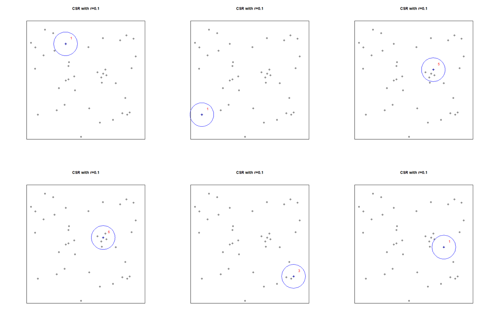
Applied Spatial Data Analysis

Chapter 2 - Second Order Statistics

Author
Affiliation

Dr. Şebnem Er

Department of Statistical Sciences, University of Cape Town

Welcome

This lecture develops second-order methods for spatial point pattern analysis.

We focus on:

  • Ripley’s \(K\) function; and
  • the pair correlation function.

Outline

  1. First- and second-order properties
  2. Morisita and Fry diagnostics
  3. Ripley’s \(K\) function
  4. Pair correlation function

First- and second-order properties

First-order structure

The first-order property of a point process is its intensity:

\[ \lambda(\mathbf{u}) = \lim_{|d\mathbf{u}|\to0} \frac{\operatorname{E}[N(d\mathbf{u})]}{|d\mathbf{u}|}. \]

It describes how the expected event density varies over space.

Second-order structure

Second-order properties describe association between pairs of events.

They address questions such as:

  • Are events unusually close together?
  • Are short interpoint distances suppressed?
  • At which distance scales does dependence occur?

Why intensity must be handled first

A pattern can look clustered because the intensity is high in one part of the region and low elsewhere, even when events are conditionally independent.

Therefore:

  1. model or estimate first-order intensity;
  2. examine residual second-order dependence;
  3. avoid attributing inhomogeneity directly to point interaction.

Quadrat-based second-order diagnostics

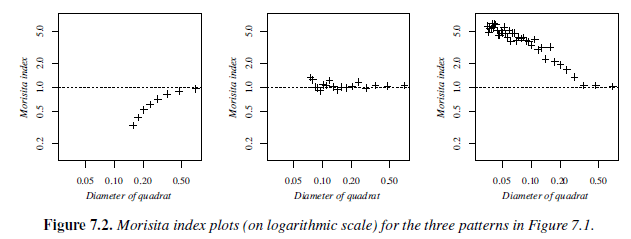
Morisita index

Suppose there are \(n\) events altogether, and there are \(n(n-1)\) number of ordered pairs of distinct events. Assume the events are divided among \(m\) quadrats with counts

\[ n_1,n_2,\ldots,n_m. \]

The number of ordered pairs in quadrat \(j\) is

\[ n_j(n_j-1). \]

The total number of ordered pairs of distinct points which fall inside the same quadrat is thus \(\sum_{j=1}^{m}n_j(n_j-1)\). The observed fraction of ordered pairs in the same quadrat is

\[ \frac{\sum_{j=1}^{m}n_j(n_j-1)}{n(n-1)}. \]

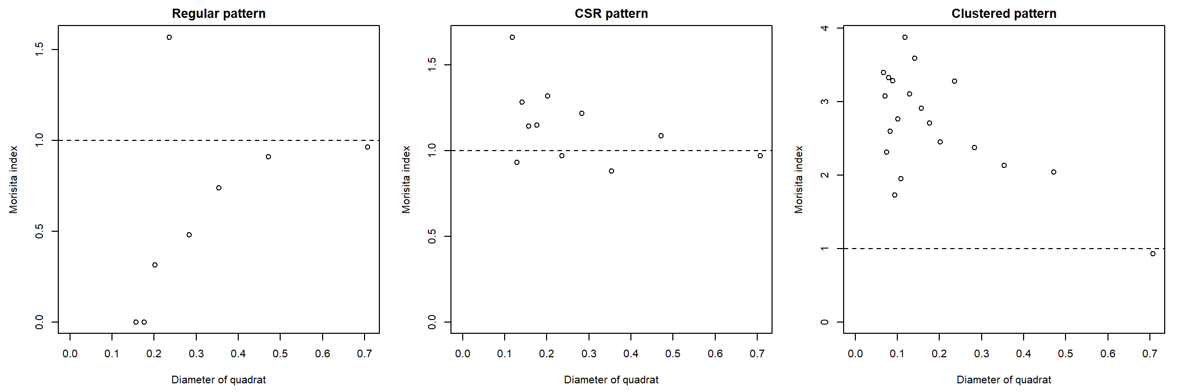
This is the fraction of all pairs of data points in which both points fall in the same quadrat. In a completely random (homogeneous Poisson) process, where points are independent of each other, two points fall in the same quadrat with probability \(1/m\), where \(m\) is the number of quadrats, so the fraction above is expected to equal \(1/m\).
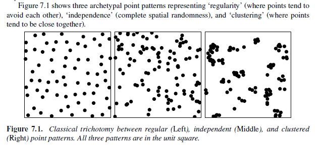
Morisita index formula

The Morisita index is

\[ I_M = m\frac{\sum_{j=1}^{m}n_j(n_j-1)}{n(n-1)}. \]

Interpretation:

  • \(I_M=1\): consistent with independence;
  • \(I_M>1\): clustering;
  • \(I_M<1\): regularity.

Ref: - Baddeley, Rubak, and Turner, Spatial Point Patterns: Methodology and Applications with R. Page:201

Ref: - Baddeley, Rubak, and Turner, Spatial Point Patterns: Methodology and Applications with R. Page:201

Morisita index in R

par(
  mfrow = c(1, 3),
  mar = c(4.5, 4.5, 2, 1)
)

miplot(
  pp_regular,
  main = "Regular pattern",
  xlab = "Diameter of quadrat",
  ylab = "Morisita index"
)

miplot(
  pp_csr,
  main = "CSR pattern",
  xlab = "Diameter of quadrat",
  ylab = "Morisita index"
)

miplot(
  pp_cluster,
  main = "Clustered pattern",
  xlab = "Diameter of quadrat",
  ylab = "Morisita index"
)

par(mfrow = c(1, 1))

Fry plot

Definition of a Fry plot

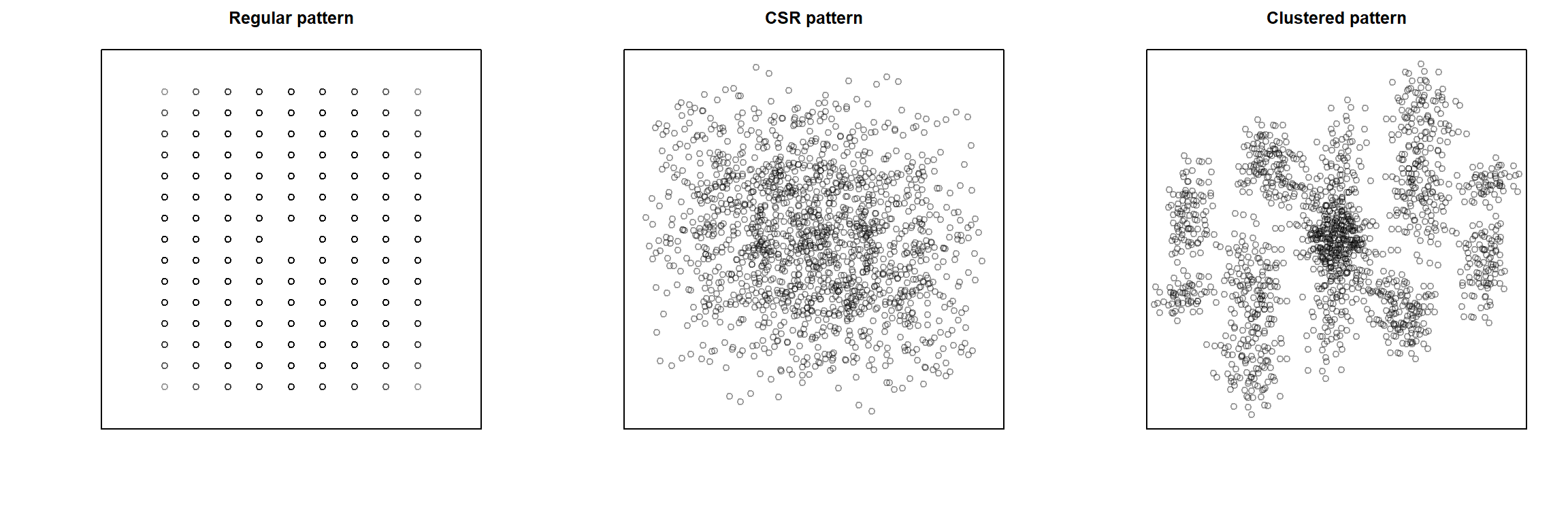
Fry plot is a scatterplot of the vector differences \(𝑥_𝑖−𝑥_𝑗\) between all pairs of distinct points in the pattern

\[ \mathbf{x}_j-\mathbf{x}_i, \]

for every ordered pair of distinct events.

The origin represents a typical event, and the plotted differences show where other events occur relative to it.

Fry plot in R

par(
  mfrow = c(1, 3),
  mar = c(4.5, 4.5, 2, 1)
)

fryplot(
  pp_regular,
  main = "Regular pattern"
)

fryplot(
  pp_csr,
  main = "CSR pattern"
)

fryplot(
  pp_cluster,
  main = "Clustered pattern"
)

par(mfrow = c(1, 1))

Ripley’s K function

Definition

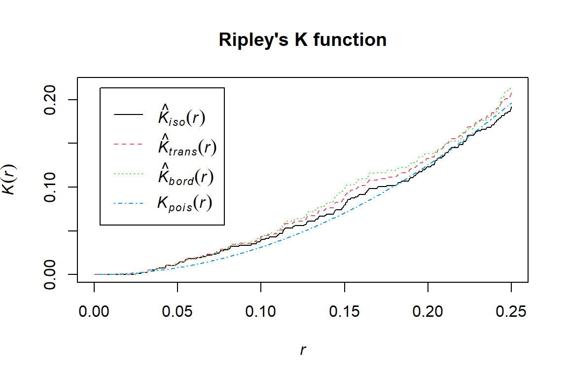
For a stationary point process with intensity \(\lambda\), Ripley’s \(K\) function is defined by

\[ K(r) = \frac{1}{\lambda} \operatorname{E} \left[N_0(r)\right]. \]

where where \(𝐸[.]\) denotes the expectation and \(𝑁_0 (𝑟)\) represents the number of further events up to a distance r around an arbitrary event.

K function under CSR

Under a homogeneous Poisson process, the expected number of further events in a disc of radius \(r\) is

\[ \lambda\pi r^2. \]

Therefore,

\[ K_{\text{CSR}}(r)=\pi r^2. \]

Empirical K function

A generic edge-corrected estimator has the form

\[ \widehat{K}(r) = \frac{|W|}{n(n-1)} \sum_{i=1}^{n} \sum_{j\ne i} \frac{\mathbf{1}(d_{ij}\le r)}{e_{ij}}, \]

where \(e_{ij}\) is an edge-correction weight.

Edge effects in K

Events near the boundary have part of their radius-\(r\) neighbourhood outside the observation window.

Without correction, their neighbour counts are systematically too small.

Common corrections include:

  • border correction;
  • translation correction;
  • isotropic correction.

K function in R

K_csr <- Kest(
  pp_csr,
  correction = c("border", "isotropic", "translate")
)
plot(K_csr, main = "Ripley's K function")

Interpreting K

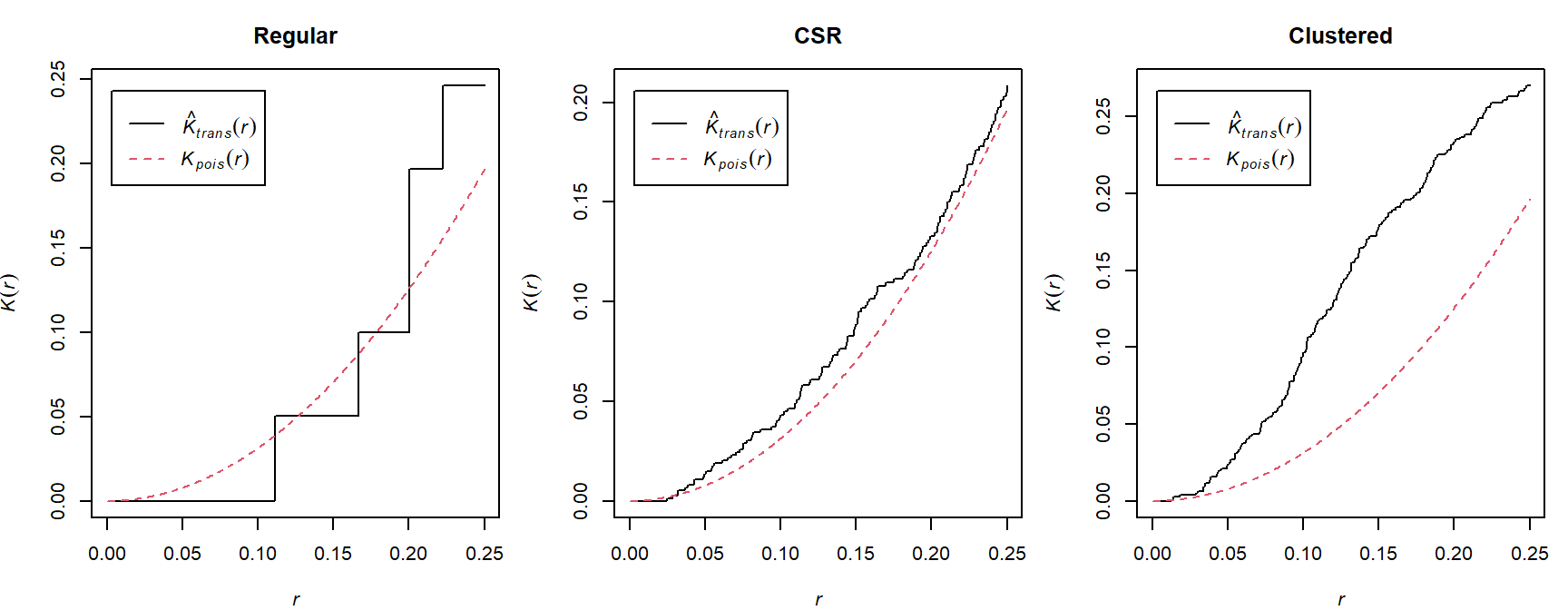
Relative to the CSR benchmark:

\[ \widehat{K}(r)>\pi r^2 \]

suggests more neighbours than expected and is consistent with clustering.

\[ \widehat{K}(r)<\pi r^2 \]

suggests fewer neighbours than expected and is consistent with inhibition or regularity.

Comparing K across patterns

Important cautions

Stationarity and inhomogeneity

The standard homogeneous versions of \(G\), \(F\), \(J\), and \(K\) assume stationarity or homogeneity.

A spatial trend in intensity can produce apparent clustering even when events are independent conditional on the trend.

For inhomogeneous patterns, consider intensity-adjusted methods such as

\[ K_{\mathrm{inhom}}(r) \]

and suitable residual diagnostics.

Edge correction

Edge correction matters because events or reference locations near the boundary have unobservable neighbourhoods outside the window.

The impact grows as the distance \(r\) increases.

Good practice:

  • report the correction used;
  • avoid over-interpreting very large distances;
  • compare corrections when results are sensitive;
  • use simulation under the same observation window.

Correlation is not causation

Second-order summaries identify spatial association, not its cause.

Similar clustering can result from:

  • environmental heterogeneity;
  • social or biological interaction;
  • dispersal mechanisms;
  • unmeasured covariates;
  • observation or sampling processes.

Summary

Main ideas

  • Nearest-neighbour distances describe spacing between events.
  • Empty-space distances describe gaps in the pattern.
  • The \(G\), \(F\), and \(J\) functions retain information across distances.
  • Ripley’s \(K\) function measures cumulative second-order structure.
  • The pair correlation function isolates structure near a particular distance.
  • Intensity and edge effects must be handled before interpreting dependence.

Reproducibility information

sessionInfo()
R version 4.4.1 (2024-06-14 ucrt)
Platform: x86_64-w64-mingw32/x64
Running under: Windows 10 x64 (build 19043)

Matrix products: default


locale:
[1] LC_COLLATE=English_United Kingdom.utf8 
[2] LC_CTYPE=English_United Kingdom.utf8   
[3] LC_MONETARY=English_United Kingdom.utf8
[4] LC_NUMERIC=C                           
[5] LC_TIME=English_United Kingdom.utf8    

time zone: Africa/Johannesburg
tzcode source: internal

attached base packages:
[1] stats     graphics  grDevices utils     datasets  methods   base     

other attached packages:
[1] spatstat.model_3.3-6   rpart_4.1.23           spatstat.explore_3.4-3
[4] nlme_3.1-164           spatstat.random_3.4-1  spatstat.geom_3.4-1   
[7] spatstat.univar_3.1-3  spatstat.data_3.1-6   

loaded via a namespace (and not attached):
 [1] cli_3.6.4             knitr_1.51            rlang_1.1.5          
 [4] spatstat.sparse_3.1-0 xfun_0.55             spatstat.utils_3.1-4 
 [7] jsonlite_2.0.0        htmltools_0.5.8.1     rmarkdown_2.29       
[10] grid_4.4.1            evaluate_1.0.5        abind_1.4-8          
[13] fastmap_1.2.0         yaml_2.3.10           compiler_4.4.1       
[16] goftest_1.2-3         polyclip_1.10-7       htmlwidgets_1.6.4    
[19] mgcv_1.9-1            rstudioapi_0.18.0     lattice_0.22-6       
[22] digest_0.6.37         tensor_1.5            splines_4.4.1        
[25] Matrix_1.7-0          tools_4.4.1           deldir_2.0-4