[,1]  [,2]  [,3]  [,4]
[1,] 0.000 0.293 0.516 0.284
[2,] 0.293 0.000 0.598 0.463
[3,] 0.516 0.598 0.000 0.255
[4,] 0.284 0.463 0.255 0.000Applied Spatial Data Analysis
Chapter 2 - Distance Based Methods
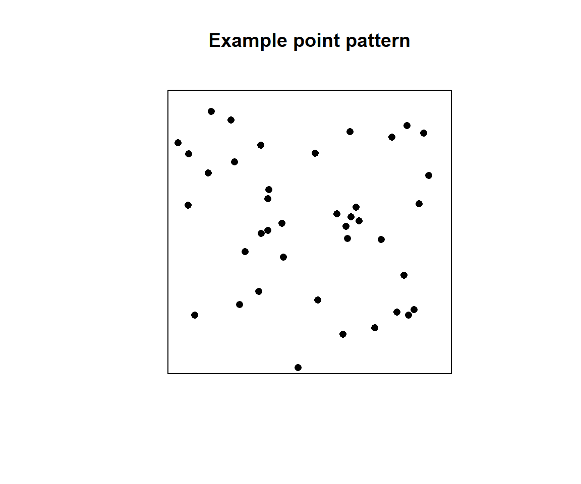
Example point pattern
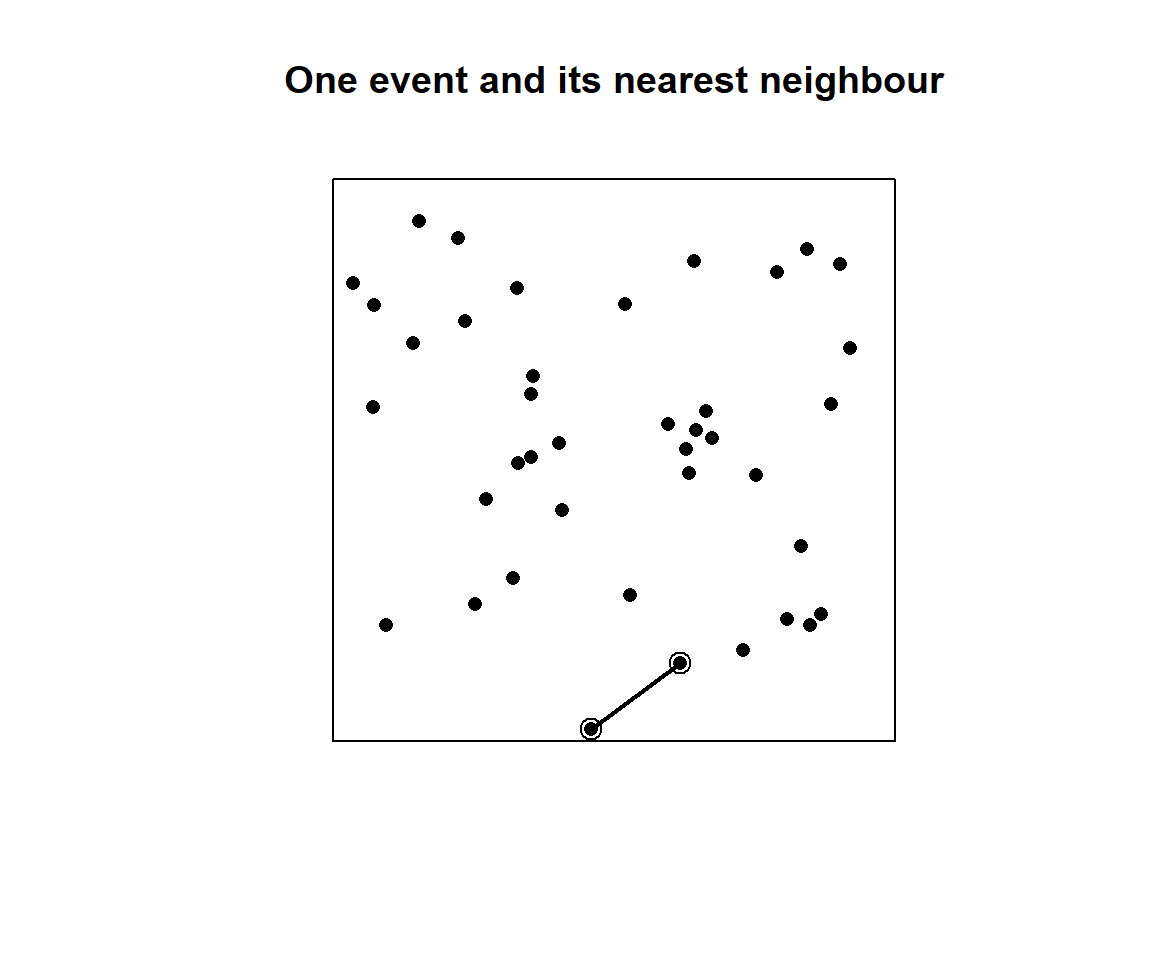
Visualising nearest neighbours
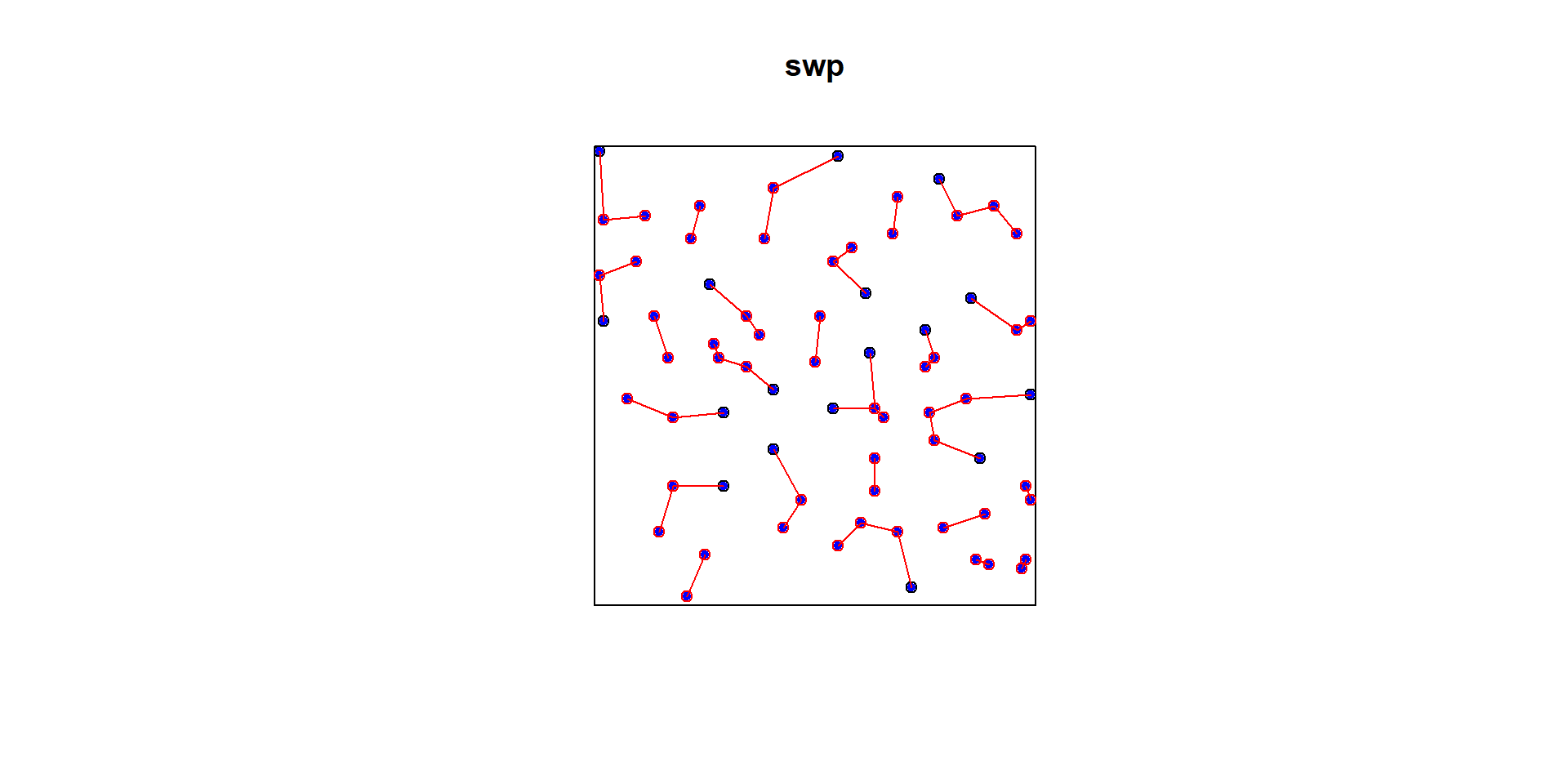
swp dataset
[1] "matrix" "array" [,1] [,2] [,3] [,4] [,5]
[1,] 0.000000 2.700000 3.701351 1.503330 5.433231
[2,] 2.700000 0.000000 1.004988 1.204159 2.765863
[3,] 3.701351 1.004988 0.000000 2.200000 1.772005
[4,] 1.503330 1.204159 2.200000 0.000000 3.931921
[5,] 5.433231 2.765863 1.772005 3.931921 0.000000R code
[1] 1.5033296 0.8544004 1.0049876 0.9055385 1.0770330 0.8544004R code
# which is the same as nndist e2e=nndist(swp)

dmin = nndist(swp)

plot(swp)
xy = cbind(swp$x, swp$y)

ord <- rev(order(dmin))
far25 <- ord[1:71]
neighbors <- wdmin[far25]
points(xy[far25, ], col='blue', pch=20)
points(xy[neighbors, ], col='red')
# drawing the lines, easiest via a loop
for (i in far25) {
    lines(rbind(xy[i, ], xy[wdmin[i], ]), col='red')
}
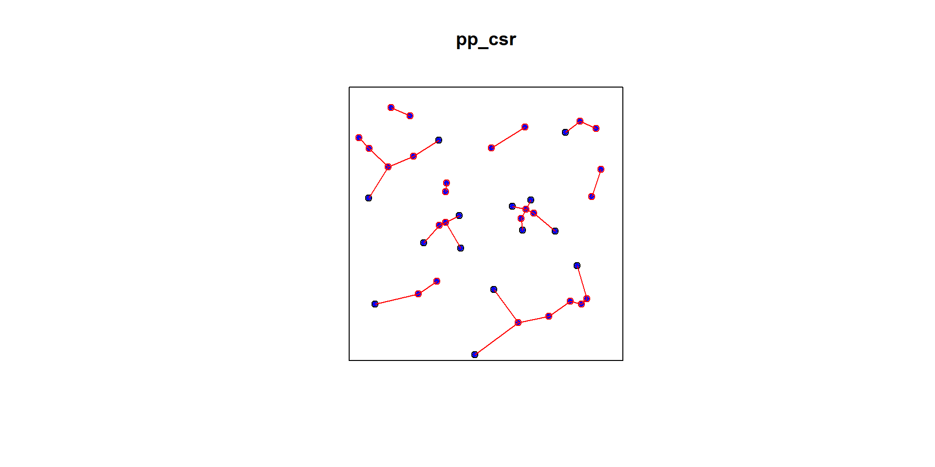
Simulated CSR Pattern
 [1] 0.11056220 0.05419105 0.08163249 0.05574520 0.19907565 0.03191166
 [7] 0.10456756 0.15049858 0.16325765 0.02841510 0.05044346 0.05419105
[13] 0.10456756 0.07525211 0.02471890 0.08651227 0.03700818 0.06471165
[19] 0.12663659 0.08163249 0.06471165 0.07525211 0.14362670 0.03195288
[25] 0.09669706 0.03195288 0.09731910 0.04284774 0.11297958 0.03191166
[31] 0.13454666 0.02841510 0.02471890 0.06711512 0.10924574 0.04269836
[37] 0.09947882 0.03815278 0.14362670 0.10235020[1] "matrix" "array" [,1] [,2] [,3] [,4] [,5]
[1,] 0.0000000 0.2930205 0.5163115 0.2844957 0.7955061
[2,] 0.2930205 0.0000000 0.5975953 0.4633681 0.8993362
[3,] 0.5163115 0.5975953 0.0000000 0.2546708 0.3017974
[4,] 0.2844957 0.4633681 0.2546708 0.0000000 0.5130861
[5,] 0.7955061 0.8993362 0.3017974 0.5130861 0.0000000R code
[1] 0.11056220 0.05419105 0.08163249 0.05574520 0.19907565 0.03191166R code
# which is the same as nndist e2e=nndist(swp)

dmin = nndist(pp_csr)

plot(pp_csr)
xy = cbind(pp_csr$x, pp_csr$y)

ord <- rev(order(dmin))
far25 <- ord[1:40]
neighbors <- wdmin[far25]
points(xy[far25, ], col='blue', pch=20)
points(xy[neighbors, ], col='red')
# drawing the lines, easiest via a loop
for (i in far25) {
    lines(rbind(xy[i, ], xy[wdmin[i], ]), col='red')
}
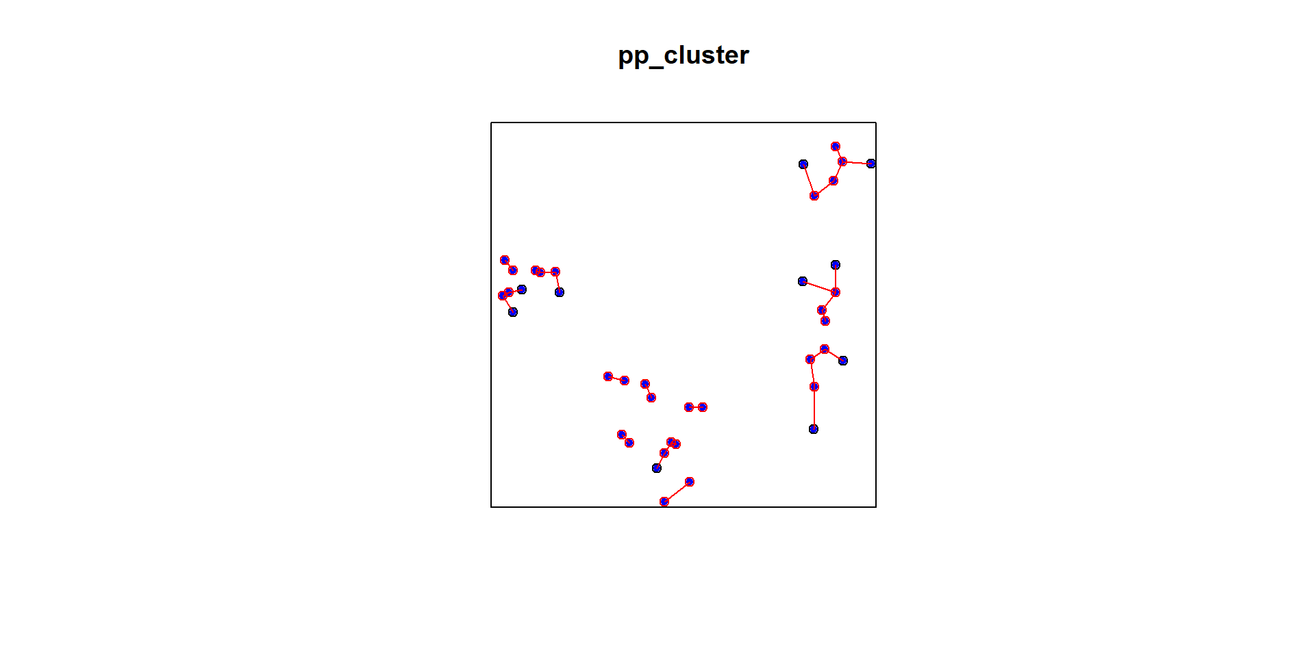
Simulated Cluster Pattern
 [1] 0.01854666 0.03502091 0.01854666 0.04969353 0.03502091 0.03390187
 [7] 0.01268286 0.05624330 0.01268286 0.03830134 0.04275255 0.02983313
[13] 0.04275255 0.02983313 0.03774271 0.03774271 0.03391843 0.01376367
[19] 0.01376367 0.03500058 0.08344093 0.06403124 0.05422191 0.08344093
[25] 0.03500058 0.08988091 0.04304986 0.07202173 0.04586212 0.02906394
[31] 0.08760076 0.11053898 0.04586212 0.02906394 0.05896243 0.07149045
[37] 0.04361429 0.04361429 0.05745563 0.07483198[1] "matrix" "array" [,1] [,2] [,3] [,4] [,5]
[1,] 0.00000000 0.09345138 0.01854666 0.04969353 0.07093497
[2,] 0.09345138 0.00000000 0.08597921 0.13688899 0.03502091
[3,] 0.01854666 0.08597921 0.00000000 0.05097721 0.05847323
[4,] 0.04969353 0.13688899 0.05097721 0.00000000 0.10757315
[5,] 0.07093497 0.03502091 0.05847323 0.10757315 0.00000000R code
[1] 0.01854666 0.03502091 0.01854666 0.04969353 0.03502091 0.03390187R code
# which is the same as nndist e2e=nndist(swp)

dmin_cluster = nndist(pp_cluster)

plot(pp_cluster)
xy_cluster = cbind(pp_cluster$x, pp_cluster$y)

ord <- rev(order(dmin_cluster))
far25 <- ord[1:40]
neighbors <- wdmin_cluster[far25]
points(xy_cluster[far25, ], col='blue', pch=20)
points(xy_cluster[neighbors, ], col='red')
# drawing the lines, easiest via a loop
for (i in far25) {
    lines(rbind(xy_cluster[i, ], xy_cluster[wdmin_cluster[i], ]), col='red')
}
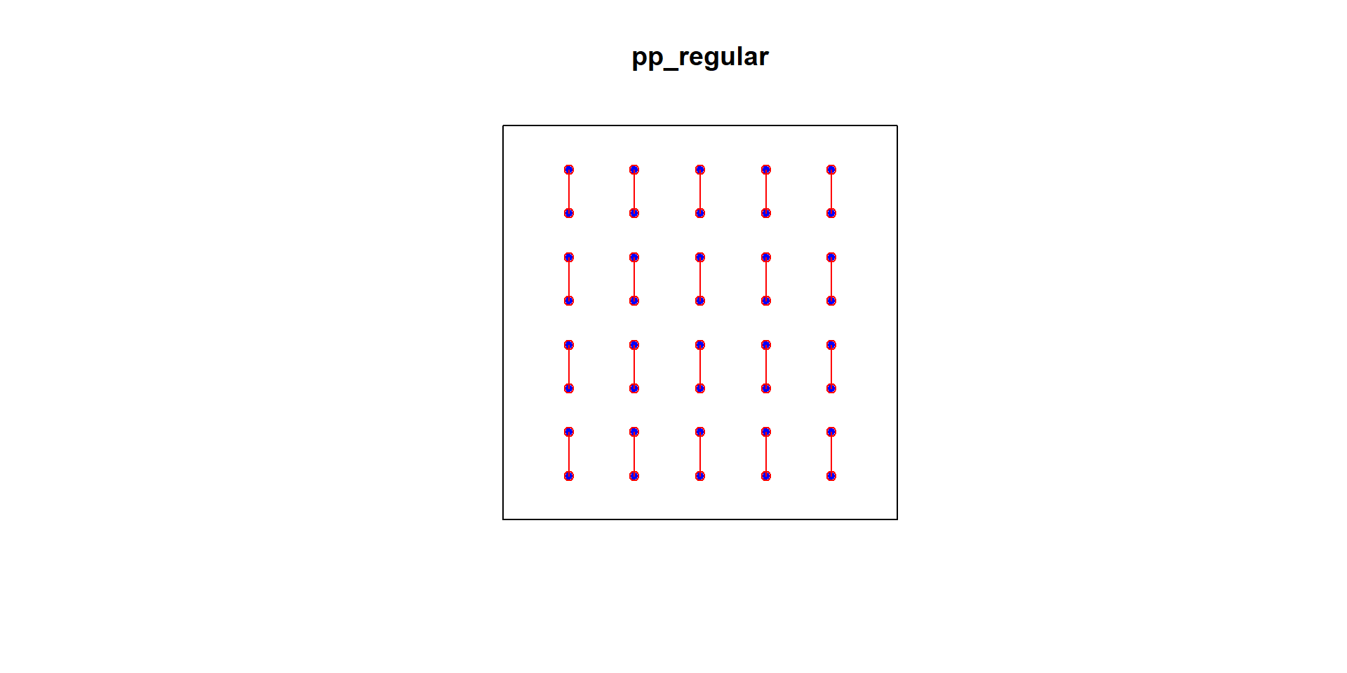
Simulated Regular Pattern
 [1] 0.1111111 0.1111111 0.1111111 0.1111111 0.1111111 0.1111111 0.1111111
 [8] 0.1111111 0.1111111 0.1111111 0.1111111 0.1111111 0.1111111 0.1111111
[15] 0.1111111 0.1111111 0.1111111 0.1111111 0.1111111 0.1111111 0.1111111
[22] 0.1111111 0.1111111 0.1111111 0.1111111 0.1111111 0.1111111 0.1111111
[29] 0.1111111 0.1111111 0.1111111 0.1111111 0.1111111 0.1111111 0.1111111
[36] 0.1111111 0.1111111 0.1111111 0.1111111 0.1111111[1] "matrix" "array" [,1] [,2] [,3] [,4] [,5]
[1,] 0.0000000 0.1666667 0.3333333 0.5000000 0.6666667
[2,] 0.1666667 0.0000000 0.1666667 0.3333333 0.5000000
[3,] 0.3333333 0.1666667 0.0000000 0.1666667 0.3333333
[4,] 0.5000000 0.3333333 0.1666667 0.0000000 0.1666667
[5,] 0.6666667 0.5000000 0.3333333 0.1666667 0.0000000R code
            X             Y
1 -0.05610447 -0.0005489143
2 -0.27914228 -0.0569200607
3 -0.41836751 -0.0294786165
4 -0.61092147 -0.0553659112
5 -0.63425768  0.0879645408
6 -0.13475501 -0.1903105666
R code
# which is the same as nndist e2e=nndist(swp)

dmin_regular = nndist(pp_regular)

plot(pp_regular)
xy_regular = cbind(pp_regular$x, pp_regular$y)

ord <- rev(order(dmin_regular))
far25 <- ord[1:40]
neighbors <- wdmin_regular[far25]
points(xy_regular[far25, ], col='blue', pch=20)
points(xy_regular[neighbors, ], col='red')
# drawing the lines, easiest via a loop
for (i in far25) {
    lines(rbind(xy_regular[i, ], xy_regular[wdmin_regular[i], ]), col='red')
}
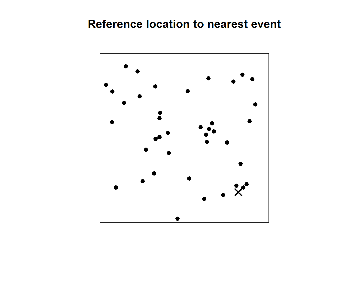
p2e distance - Point-to-event distance
For an arbitrary reference location \(\mathbf{u}\), the empty-space distance is
\[ E(\mathbf{u})=\min_i\lVert\mathbf{u}-\mathbf{x}_i\rVert. \]
Other indices
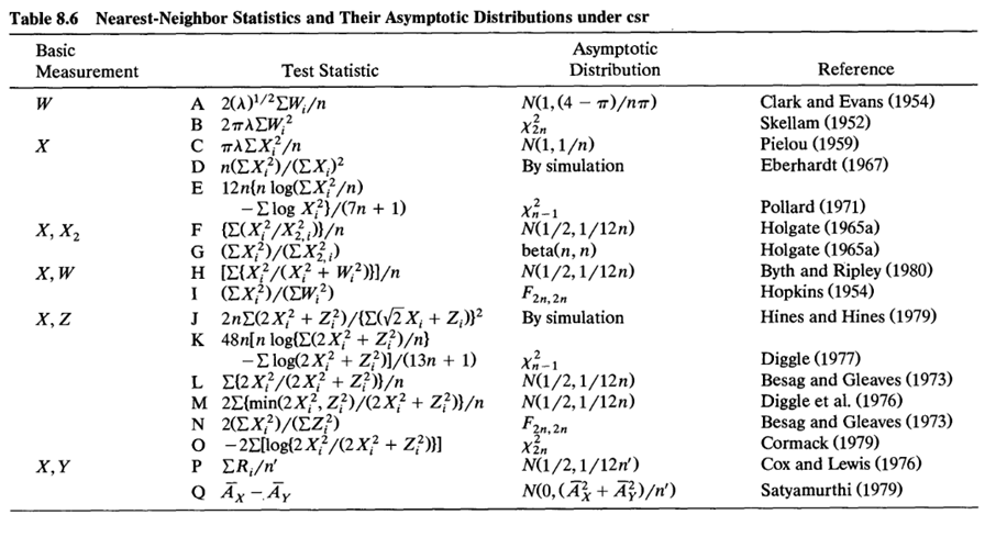
Ref: Noel Cressie, (1991). Statistics for Spatial Data, Wiley, page604.
The G and F functions - Observed and Expected Distributions of e2e and p2e distances
For a homogeneous Poisson process with intensity \(\lambda\), the probability that a disc of radius \(r\) contains no events is
\[ \Pr\{N(A(\mathbf{u},r))=0\}=\exp(-\lambda\pi r^2). \]
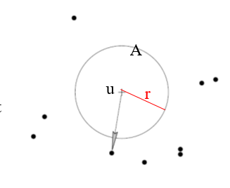
\[ \Pr\{d(u,X)>r\}=\Pr \{n(X \cap a(u,r))=0\}=\exp(-\lambda\pi r^2) \]
Therefore,
\[ 1-\exp(-\lambda\pi r^2) \]
is the probability that at least one event lies within distance \(r\).
G function - Cumulative frequency distribution of nearest neighbourhood distances
The nearest-neighbour distribution function is
\[ G(r)=\Pr(D\le r). \]
It is the proportion of observed events whose nearest neighbour is no farther than \(r\).
Under CSR,
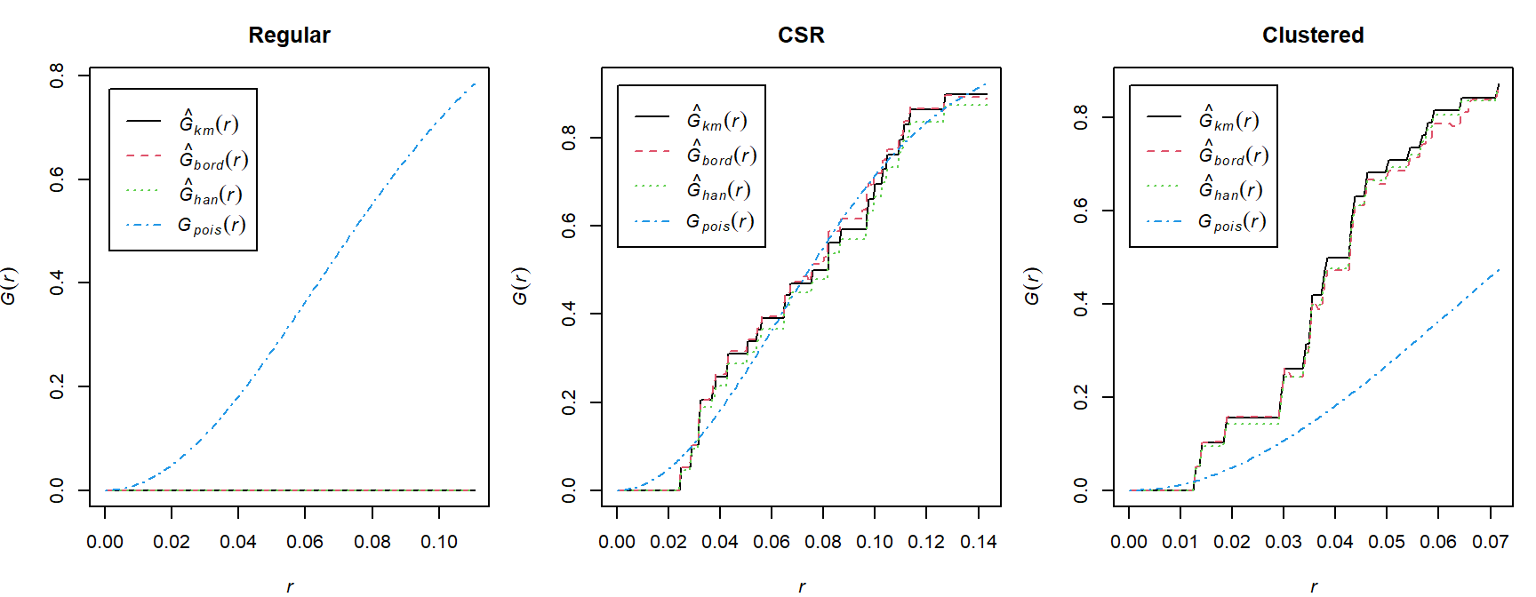
\[ G_{\text{CSR}}(r)=1-\exp(-\lambda\pi r^2). \]
Manual empirical G function
The empirical nearest-neighbour distribution function is
\[ \hat{G}(r) = \frac{1}{n} \sum_{i=1}^{n} I(D_i \le r), \]
where the indicator function is defined as
\[ I(D_i \le r) = \begin{cases} 1, & \text{if } D_i \le r, \\ 0, & \text{otherwise}. \end{cases} \]
Thus, \(\hat{G}(r)\) is simply the proportion of nearest-neighbour distances that are less than or equal to \(r\). It is the empirical cumulative distribution function (ECDF) of the nearest-neighbour distances.
- First calculate the unique nearest neighbour distances between events.
- Sort them from smallest to largest.
 [1] 0.00000000 0.02471890 0.02841510 0.03191166 0.03195288 0.03700818
 [7] 0.03815278 0.04269836 0.04284774 0.05044346 0.05419105 0.05574520
[13] 0.06471165 0.06711512 0.07525211 0.08163249 0.08651227 0.09669706
[19] 0.09731910 0.09947882 0.10235020 0.10456756 0.10924574 0.11056220
[25] 0.11297958 0.12663659 0.13454666 0.14362670 0.15049858 0.16325765
[31] 0.19907565- Count how many events exist that are less than the distances (either empirical or chosen at an interval - I will use interval (0-max dist) with small increments). (This could be achieved using
plot(Gest())function in R. Always a good practice to do this manually first.)
R code
       r    G
1  0.000 0.00
2  0.005 0.00
3  0.010 0.00
4  0.015 0.00
5  0.020 0.00
6  0.025 0.05
7  0.030 0.10
8  0.035 0.20
9  0.040 0.25
10 0.045 0.30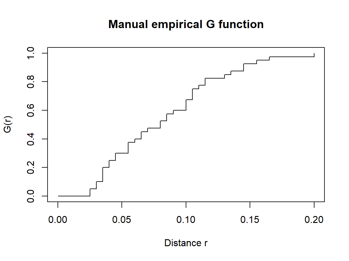
G function using spatstat
R code
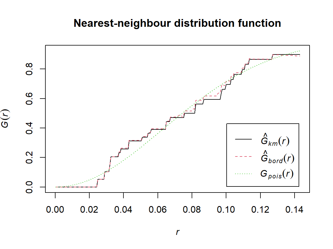
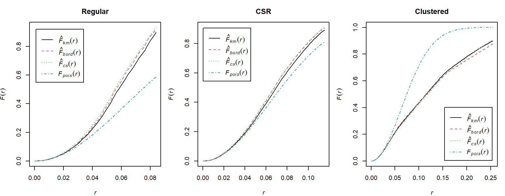
Comparing G across patterns
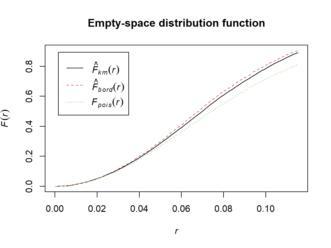
F function - Cumulative frequency distribution of distance E from an arbitrary point to the nearest (other) event - Empty-space distribution function F
The empty-space function is
\[ F(r)=\Pr(E\le r). \]
It is the proportion of locations in the study region that lie within distance \(r\) of an event.
Let
\[ E_1,E_2,\ldots,E_m \]
be the distances from \(m\) randomly selected locations in the study region to their nearest event.
The empirical empty-space function is defined as
\[ \hat{F}(r) = \frac{1}{m} \sum_{i=1}^{m} I(E_i \le r), \]
where the indicator function is
\[ I(E_i \le r) = \begin{cases} 1, & \text{if } E_i \le r, \\ 0, & \text{otherwise}. \end{cases} \]
Thus, \(\hat{F}(r)\) is simply the proportion of randomly selected locations whose nearest event is within a distance \(r\). Equivalently, it is the empirical cumulative distribution function (ECDF) of the point-to-event (empty-space) distances.
In practice, the distances
\[ E_1,E_2,\ldots,E_m \]
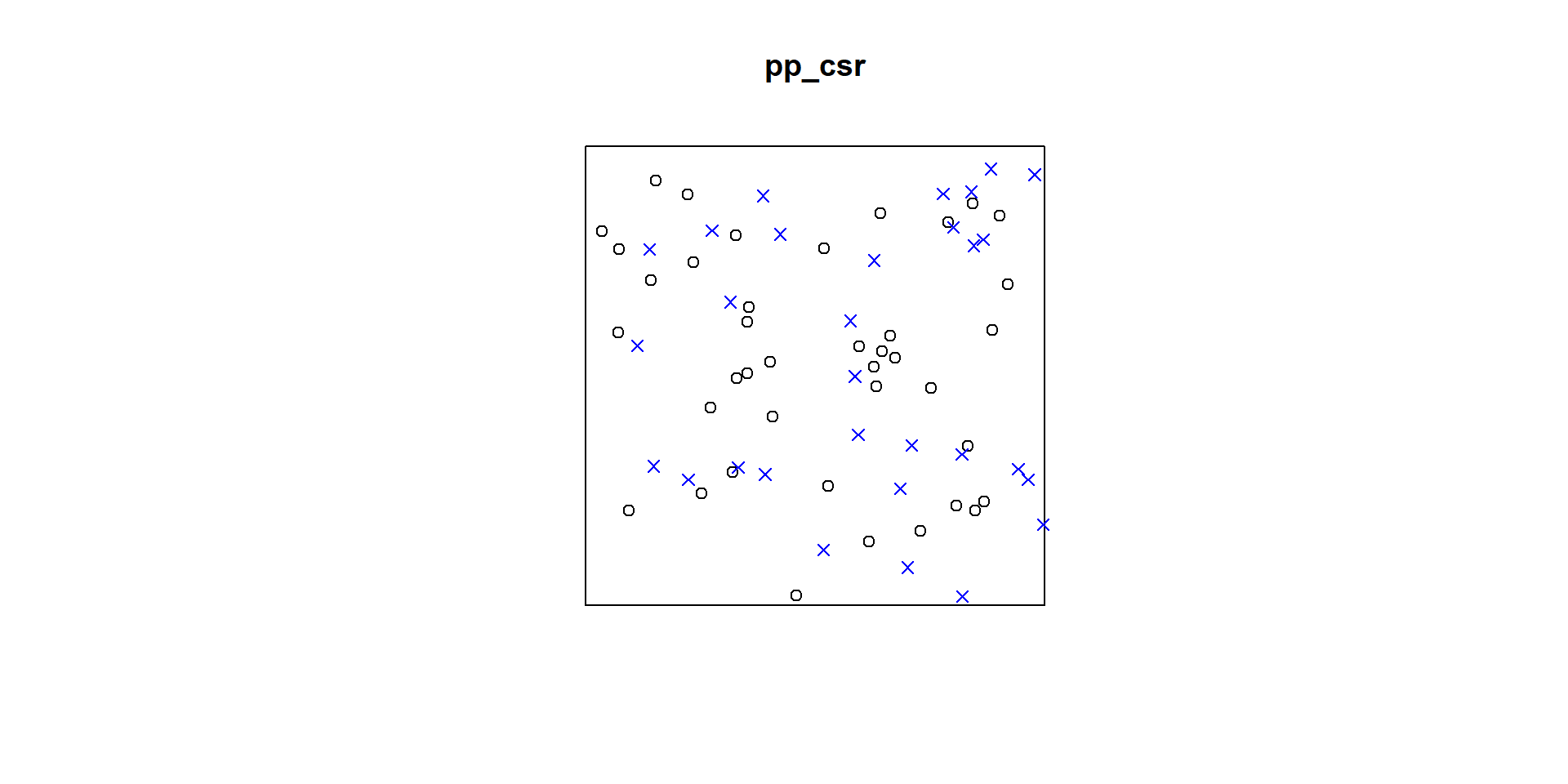
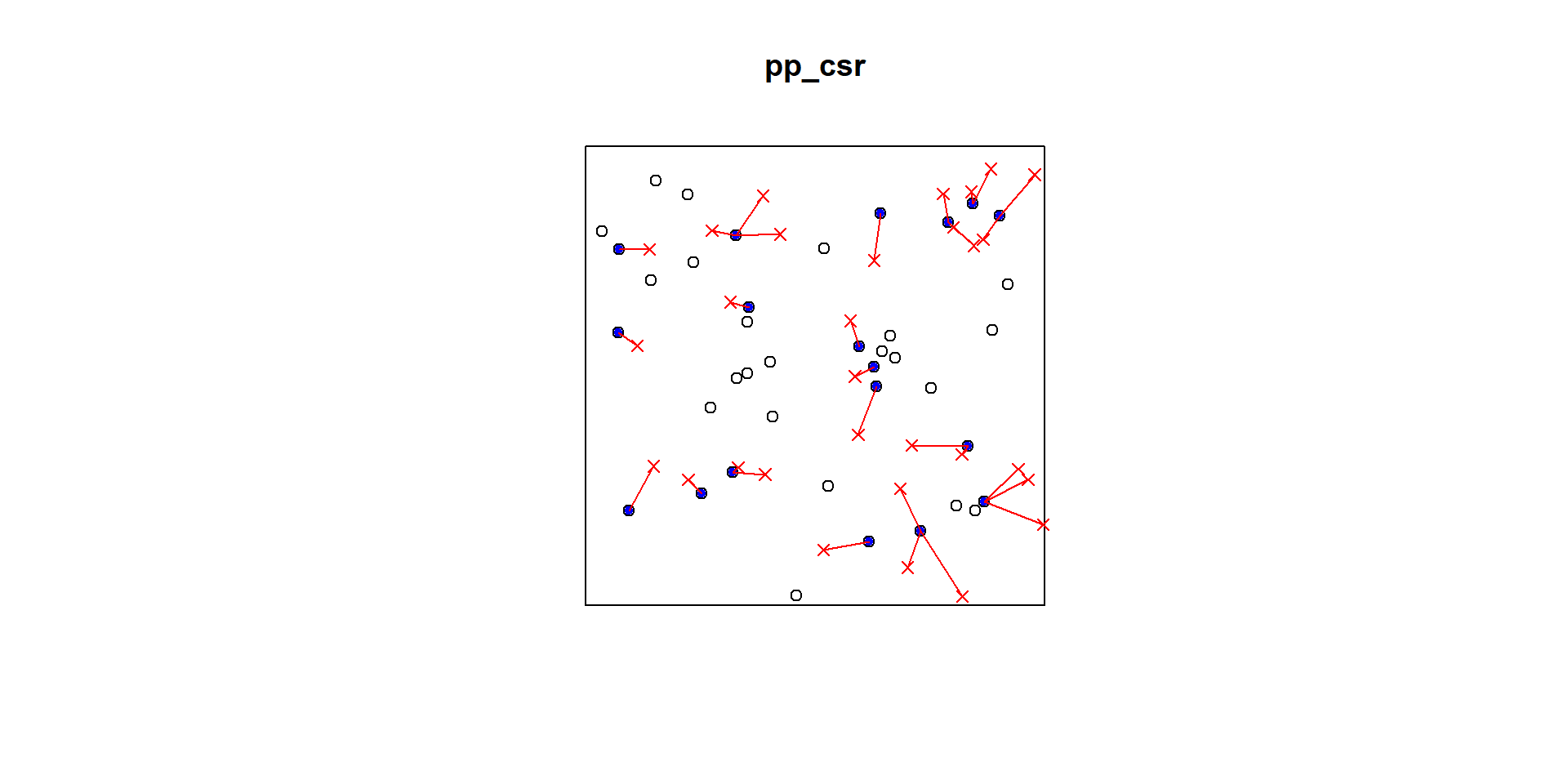
are obtained by generating a large number of random locations uniformly over the study region and computing the distance from each location to its nearest observed event.
Under CSR,
\[ F_{\text{CSR}}(r)=1-\exp(-\lambda\pi r^2). \]
Manual approximation to F
R code
R code
p2e_distances_csr = NULL
mins_csr = NULL
xy = cbind(pp_csr$x, pp_csr$y)


# sqrt((xy[2,1]-randompoints[1,1])^2+(xy[2,2]-randompoints[1,2])^2)
# sqrt((xy[1,1]-randompoints[2,1])^2+(xy[1,2]-randompoints[2,2])^2)


for(i in 1:dim(randompoints)[1]){
dist1 = matrix(pairdist(rbind(randompoints[i,],xy)),41)

p2e_distances_csr = c(p2e_distances_csr,min(dist1[2:41,1]))
mins_csr = c(mins_csr,which.min(dist1[2:41,1]))
}


plot(pp_csr)
ord <- rev(order(p2e_distances_csr))
far25 <- 1:dim(randompoints)[1]
neighbors <- mins_csr
points(randompoints, col='red', pch=4)
points(xy[mins_csr, ], col='blue', pch=20)
# drawing the lines, easiest via a loop
for (i in far25) {
  lines(rbind(xy[mins_csr[i], ], randompoints[i, ]), col='red')
}
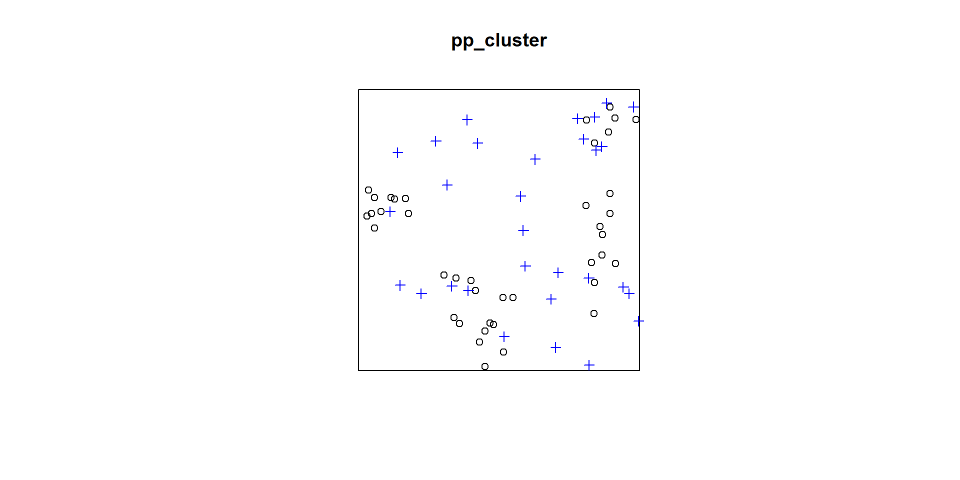
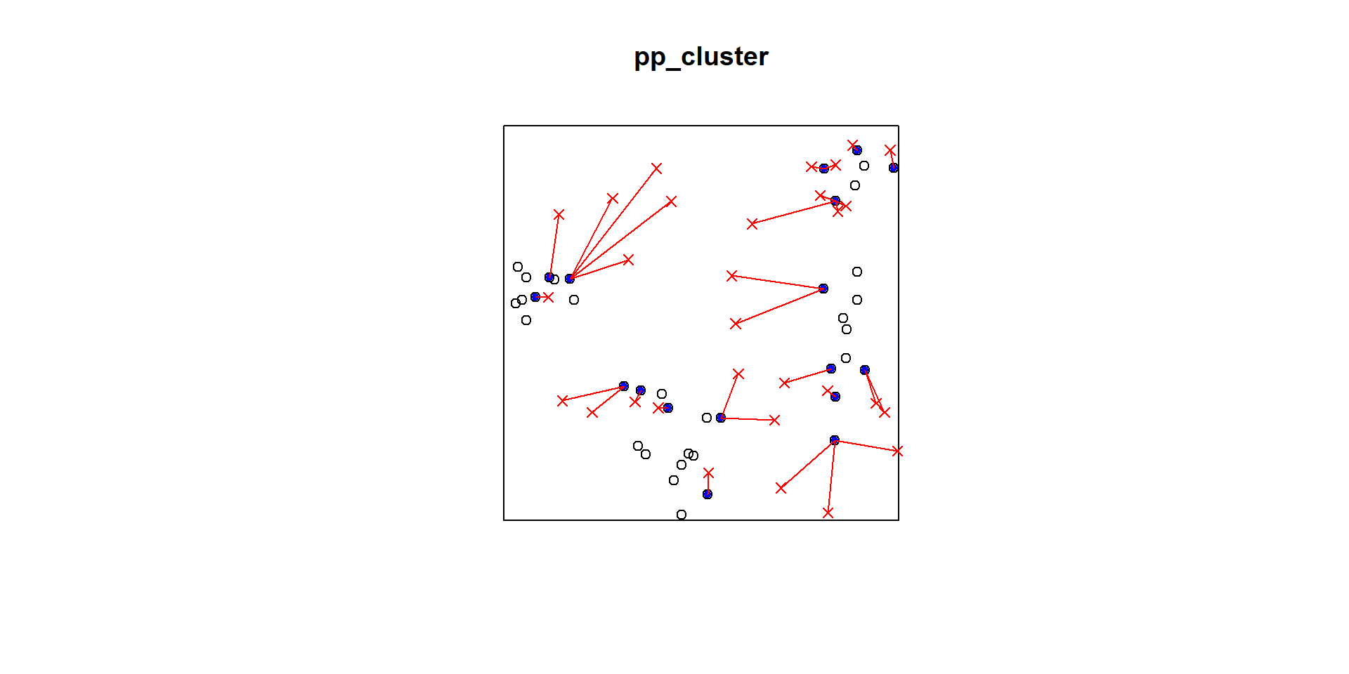
Cluster Pattern
R code
p2e_distances_cluster = NULL
mins_cluster = NULL
xy_cluster = cbind(pp_cluster$x, pp_cluster$y)

for(i in 1:dim(randompoints)[1]){
dist1 = matrix(pairdist(rbind(randompoints[i,],xy_cluster)),41)

p2e_distances_cluster = c(p2e_distances_cluster,min(dist1[2:41,1]))
mins_cluster = c(mins_cluster,which.min(dist1[2:41,1]))
}


plot(pp_cluster)
ord <- rev(order(p2e_distances_cluster))
far25 <- 1:dim(randompoints)[1]
neighbors <- mins_cluster
points(randompoints, col='red', pch=4)
points(xy_cluster[mins_cluster, ], col='blue', pch=20)
# drawing the lines, easiest via a loop
for (i in far25) {
  lines(rbind(xy_cluster[mins_cluster[i], ], randompoints[i, ]), col='red')
}
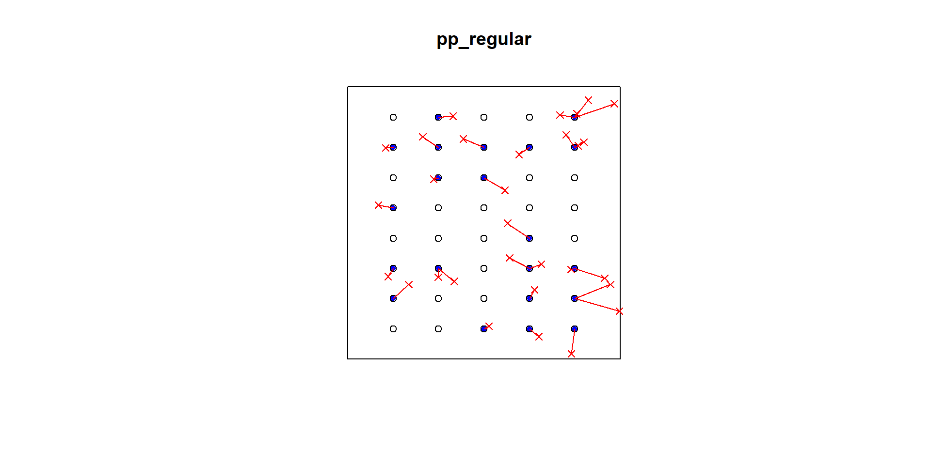
Regular Pattern
R code
p2e_distances_regular = NULL
p2e_mins_regular = NULL
xy_regular = cbind(pp_regular$x, pp_regular$y)


for(i in 1:dim(randompoints)[1]){
dist1 = matrix(pairdist(rbind(randompoints[i,],xy_regular)),41)

p2e_distances_regular = c(p2e_distances_regular,min(dist1[2:41,1]))
p2e_mins_regular = c(p2e_mins_regular,which.min(dist1[2:41,1]))
}


plot(pp_regular)
ord <- rev(order(p2e_distances_regular))
far25 <- 1:dim(randompoints)[1]
neighbors <- p2e_mins_regular
points(randompoints, col='red', pch=4)
points(xy_regular[p2e_mins_regular, ], col='blue', pch=20)
# drawing the lines, easiest via a loop
for (i in far25) {
  lines(rbind(xy_regular[p2e_mins_regular[i], ], randompoints[i, ]), col='red')
}
F function using spatstat
R code
Comparing F across patterns
J function
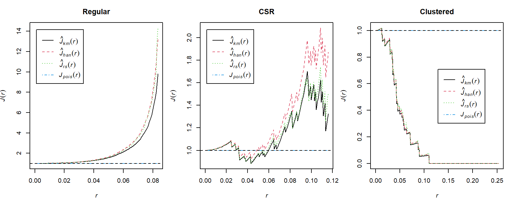
Nearest-neighbour distances and empty-space distances have the same probability distribution if the pattern is completely random. Under various departures from complete spatial randomness, the nearest-neighbour and empty-space distances tend to respond in opposite directions — one becoming larger while the other becomes smaller.
This suggests that a comparison of these two types of distance could be useful in assessing departure from CSR. A useful combination of F and G, suggested by fundamental theory, is the J-function [663] of a stationary point process,
The \(J\) function combines \(F\) and \(G\):
\[ J(r)=\frac{1-G(r)}{1-F(r)}, \]
defined for all \(r\geq0\) for distances where
\[ F(r)<1. \]
Under CSR,
\[ J_{pois}(r)\equiv 1\\ F_{pois}(r)\equiv G_{pois}(r) \]
Interpreting J
- \(J(r)>1\): consistent with regularity at scale \(r\);
- \(J(r)<1\): consistent with clustering at scale \(r\);
- \(J(r)\approx1\): consistent with CSR at scale \(r\).
Simulation envelopes
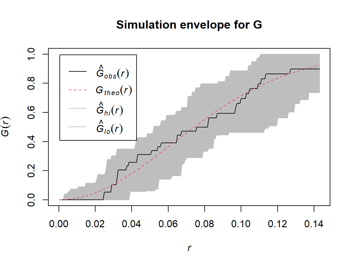
A visual comparison with a theoretical curve does not account for random variation. Simulation envelopes provide a reference band under a fitted null model.
R code