Chapter 1



Overview of Applied Spatial Data Analysis (ASDA)

Reading

Applied Spatial Data Analysis - Lecture 1: Introduction

Course information

The course introduces you to statistical techniques designed to analyse spatial data where location of observations is important. The course is intended to be practically oriented, with an emphasis on applied learning through worked examples and case studies.

Learning Outcomes

Learning Outcomes

• Identify and distinguish key types of spatial data (point patterns, geostatistical, areal/lattice)
• Understand spatial dependence and spatial autocorrelation in analysis and modelling of spatial data
• Explore spatial patterns using Exploratory Spatial Data Analysis techniques
• Select and justify appropriate methods for different spatial problems
• Apply spatial methods using R
• Interpret and communicate spatial analysis results and insights
• Engage critically with spatial statistics literature
• Recognise and address common challenges in spatial data analysis

📖 Core Resources

Lecture notes/slides will be primarily based on material presented in the following textbooks:

• 📖 Applied Spatial Data Analysis with R by Roger Bivand, Edzer Pebesma and Virgilio Gómez-Rubio
  • Companion site
• 📖 Geocomputation with R by Robin Lovelace, Jakub Nowosad, Jannes Muenchow
• 📖 Spatial Statistics for Data Science: Theory and Practice with R by Paula Moraga
• 📖 Spatial Point Patterns Methodology and Applications with R by Adrian Baddeley, Ege Rubak and Rolf Turner
• 📖 Spatial Data Science by Edzer Pebesma and Roger Bivand

Complementary Resources

Main: Cressie, Noel (1991). Statistics for Spatial Data. Wiley.

1. Anselin, L. (1999). Spatial Econometrics: Methods and Models. Kluwer Academic Publishers.

2. Arbia, G. (2014). A Primer for Spatial Econometrics: With Applications in R. Palgrave Macmillan UK.
   Available through the UCT Library online resources.

3. Haining, R. (2004). Spatial Data Analysis: Theory and Practice. Cambridge University Press.

4. Baddeley, A., Rubak, E., & Turner, R. (2016). Spatial Point Patterns: Methodology and Applications with R. Chapman & Hall/CRC.

   Online chapter resource: https://azaieznotesblog.files.wordpress.com/2017/08/spatial-point-patterns_chapman-hall-crc-2016.pdf

5. Wiegand, T., & Moloney, K. A. (2014). Handbook of Spatial Point-Pattern Analysis in Ecology. Chapman & Hall/CRC.
   Available through the UCT Library online resources.

6. Elhorst, P. J. (2014). Spatial Econometrics: From Cross-Sectional Data to Spatial Panels. Springer Berlin.

7. Gelfand, A. E., Diggle, P., Guttorp, P., Fuentes, M., & Fitzmaurice, G. (2010). Handbook of Spatial Statistics. Chapman & Hall/CRC.
   Available through the UCT Library online resources. Part 4 is especially useful for spatial point processes.

8. GeoDa Center. GeoDa Documentation and Learning Resources.
   https://geodacenter.github.io/

Suggested Reading Strategy

For this course, use the readings as follows:

• Conceptual foundation: Haining (2004) and Anselin (1999)
• Spatial econometrics in R: Arbia (2014) and Elhorst (2014)
• Point pattern analysis: Baddeley, Rubak, and Turner (2016)
• Advanced reference: Gelfand et al. (2010)
• Software and practice: GeoDa Center resources

R Packages Connected to the Readings

# Core spatial data handling and maps
library(sf)
library(terra)
library(tmap)
library(leaflet)
library(dplyr)

# Spatial dependence and spatial regression
library(spdep)
library(spatialreg)

# Spatial point patterns
library(spatstat.geom)
library(spatstat.explore)
library(spatstat.model)
library(deldir)

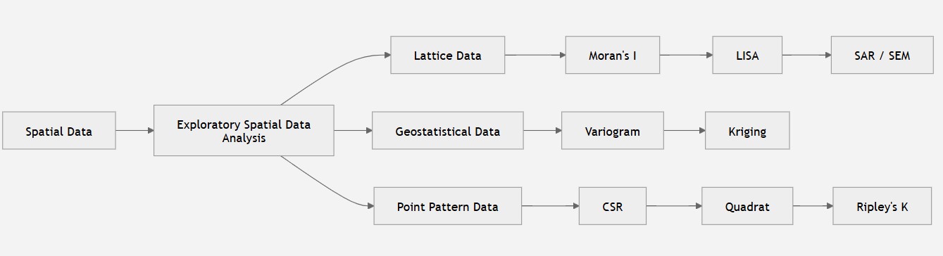
Course outline

What is Spatial Data?

• Data about the locations and shapes of geographic features and the relationships between them. These are typically stored as coordinates and topology
• Coordinates are usually two-dimensional (x,y) but can also be three-dimensional (x,y,z)
• A coordinate reference system (CRS) is typically attached to describe which location on Earth the coordinates refer to.

Data can also be:

• observational or experimental,
• continuous or categorical,
• univariate or multivariate

Historical Examples of Spatial Data

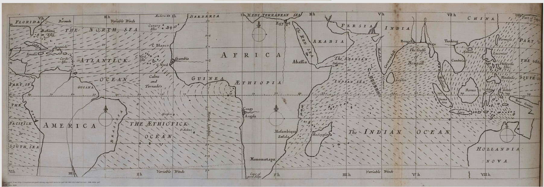
One of the first few spatial datasets appeared as maps. Examples:

Edmond Halley’s trade winds in 1686:

John Snow’s Cholera Map 1854 Broad Street, London

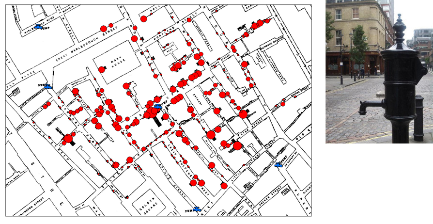
John Snow Pub in London:

Me at the pump:

Edward Tufte’s map displays

Modern examples

popup = c("Robin", "Jakub", "Jannes")
leaflet() |>
  addProviderTiles("NASAGIBS.ViirsEarthAtNight2012") |>
  addMarkers(lng = c(-3, 23, 11),
             lat = c(52, 53, 49), 
             popup = popup)

Examples from South Africa

South Africa Crime Map::

South Africa Traffic Data:

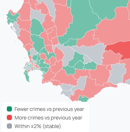
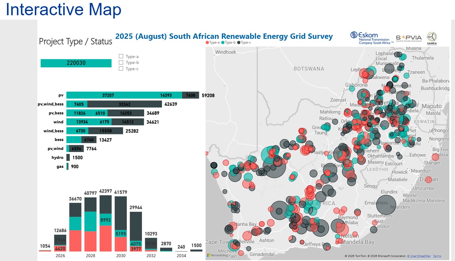
South African Renewable Energy Type Spatial Distribution:

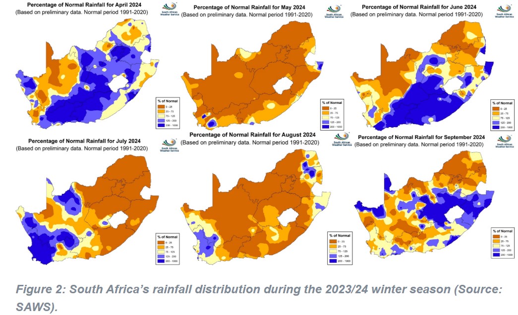
South Africa’s rainfall distribution during the 2023/24 winter season

Seasonal weather maps:

Why Spatial Analysis?

• Bivand et. al (2013): Spatial data analysis is concerned with questions about the hypothetical processes that generate the observed data.

Possible questions that may arise include the following:

• Does the spatial patterning of disease incidences give rise to the conclusion that they are clustered, and if so, are the clusters found
• Given a number of observed soil samples, which part of a study area is polluted?
• Given scattered air quality measurements, how many people are exposed to high levels of black smoke or particulate matter (e.g. PM 10 ), and where do they live?
• Do governments tend to compare their policies with those of their neighbours, or do they behave independently?

Methodological Challenges:

Spatial data can be thought of as resulting from observations of a stochastic process (Cressie, 1991):

\[ \left\{ Z(\mathbf{s}) : \mathbf{s} \in D \right\}, \qquad D \subset \mathbb{R}^d. \]

where the domain \(D\) is a set of \(\mathbb{R}^d\), usually in \(d=2\), and \(Z(s)\) denotes the attribute we observe at \(\mathbf{s}\). Spatial observations violate the foundational i.i.d. assumption of classical statistics due to spatial dependence (\(\text{Cov}(Z(\mathbf{s}_i), Z(\mathbf{s}_j)) \neq 0\)).

• Spatial Autocorrelation/Dependence: Near observations are more correlated than distant ones.

Tobler’s first law of geography:

“everything is related to everything else, but near things are more related than distant things” Waldo R. Tobler (Tobler 1970).

Mean Estimation

Consider the following simple statistical model, commonly introduced in beginning statistics courses.

Suppose

\[ Z(1), \ldots, Z(n) \]

are independent and identically distributed from a Gaussian distribution:

\[ Z(i) \overset{\text{i.i.d.}}{\sim} \mathcal{N}(\mu,\sigma_0^2), \qquad i=1,\ldots,n, \]

where

• \(\mu\) is unknown;
• \(\sigma_0^2\) is known.

The minimum-variance unbiased estimator of \(\mu\) is

\[ \bar{Z} = \frac{1}{n} \sum_{i=1}^{n} Z(i). \]

Estimation under Independence

Assume

\[ Z(1),\ldots,Z(n) \]

are independent and identically distributed,

\[ Z(i)\overset{\text{i.i.d.}}{\sim}\mathcal{N}(\mu,\sigma_0^2), \qquad i=1,\ldots,n. \]

The minimum-variance unbiased estimator of the population mean is the sample mean,

\[ \boxed{ \bar Z=\frac{1}{n}\sum_{i=1}^{n}Z(i) } \]

Since the observations are independent,

\[ \bar Z\sim\mathcal N\left(\mu,\frac{\sigma_0^2}{n}\right). \]

A two-sided 95% confidence interval for the mean is

\[ \boxed{ \bar Z\pm1.96\frac{\sigma_0}{\sqrt n} } \]

What Happens if the Observations are Correlated?

The independence assumption is no longer valid.

Suppose nearby observations are positively correlated:

\[ \operatorname{cov}\left(Z(i),Z(j)\right) = \sigma_0^2\rho^{|i-j|}, \qquad 0<\rho<1. \]

This covariance decreases as the distance between observations increases.

• If \(\rho=0\), observations are independent.
• Larger values of \(\rho\) imply stronger spatial dependence.

Effect on the Variance of the Sample Mean

Under spatial dependence,

\[ \operatorname{var}(\bar Z) = \frac{1}{n^2} \sum_{i=1}^{n} \sum_{j=1}^{n} \operatorname{cov}(Z(i),Z(j)). \]

Substituting the covariance model gives

\[ \operatorname{var}(\bar Z) = \frac{\sigma_0^2}{n} \left[ 1+ 2\left(\frac{\rho}{1-\rho}\right) \left(1-\frac1n\right) - 2 \left(\frac{\rho}{1-\rho}\right)^2 \frac{1-\rho^{\,n-1}}{n} \right]. \]

Basically, the variance is larger than under independence.

Why Does This Matter?

Suppose

• \(n=10\)
• \(\rho=0.26\)

Then

\[ \operatorname{var}(\bar Z) = \frac{\sigma_0^2}{10}(1.608). \]

Instead of

\[ 1.96\frac{\sigma_0}{\sqrt{10}}, \]

the correct multiplier becomes

\[ 2.485\frac{\sigma_0}{\sqrt{10}}. \]

Therefore the correct 95% confidence interval is

\[ \boxed{ \bar Z \pm 2.485 \frac{\sigma_0}{\sqrt{10}} } \]

which is considerably wider than the interval obtained by assuming independence.

Linear Models with Spatially Dependent Errors

Suppose observations are collected at spatial locations

\[ \mathbf{s}_1,\mathbf{s}_2,\ldots,\mathbf{s}_n, \]

where each observation is generated by the spatial process

\[ \boxed{ Z(\mathbf{s}) = \sum_{l=1}^{q}\beta_l x_l(\mathbf{s}) + \delta(\mathbf{s}), \qquad \mathbf{s}\in D\subset\mathbb{R}^d } \]

where

• \(x_l(\mathbf{s})\) is the \(l\)-th explanatory variable measured at location \(\mathbf{s}\);
• \(\beta_l\) is the corresponding regression coefficient;
• \(\delta(\mathbf{s})\) is the random error term, which may exhibit spatial dependence.

Interpretation

This model is simply a spatial extension of ordinary linear regression.

Recall the familiar regression model

\[ Y_i=\beta_0+\beta_1X_{i1}+\cdots+\beta_qX_{iq}+\varepsilon_i. \]

The spatial model replaces the independent observations with observations indexed by location,

\[ Z(\mathbf{s}) = \sum_{l=1}^{q}\beta_l x_l(\mathbf{s}) + \delta(\mathbf{s}). \]

The important difference is that

\[ \delta(\mathbf{s}) \]

may be spatially correlated.

Matrix Representation

Collect the observations into a vector

\[ \mathbf{Z} = \begin{bmatrix} Z(\mathbf{s}_1)\\ Z(\mathbf{s}_2)\\ \vdots\\ Z(\mathbf{s}_n) \end{bmatrix}. \]

Likewise define

• the design matrix \(\mathbf{X}\),
• the regression coefficients \(\boldsymbol{\beta}\),
• the spatial error vector \(\boldsymbol{\delta}\).

The model becomes

\[ \boxed{ \mathbf{Z} = \mathbf{X}\boldsymbol{\beta} + \boldsymbol{\delta} } \]

Components of the Model

\[ \mathbf{Z} = \mathbf{X}\boldsymbol{\beta} + \boldsymbol{\delta} \]

where

• \(\mathbf{Z}\) is the vector of observed responses;
• \(\mathbf{X}\) is the \(n\times q\) matrix of explanatory variables;
• \(\boldsymbol{\beta}\) contains the regression coefficients;
• \(\boldsymbol{\delta}\) contains the spatially correlated errors.

Why is this Important?

Ordinary Least Squares assumes

\[ \boldsymbol{\delta} \sim N(0,\sigma^2\mathbf{I}), \]

meaning the errors are independent.

Spatial data rarely satisfy this assumption.

Instead,

\[ \operatorname{Cov}(\boldsymbol{\delta}) = \boldsymbol{\Sigma}, \]

where

\[ \boldsymbol{\Sigma}\neq\sigma^2\mathbf{I}. \]

Neighbouring observations often have correlated errors.

South African Example

Suppose we model the percentage of households with internet access in Cape Town wards.

\[ \text{Internet Access} = \beta_0 + \beta_1(\text{Income}) + \beta_2(\text{Education}) + \beta_3(\text{Population Density}) + \delta(\mathbf{s}) \]

Even after accounting for these variables, neighbouring wards may still have similar unexplained characteristics.

This remaining spatial dependence is captured by

\[ \delta(\mathbf{s}). \]

Ignoring spatial dependence leads to

• underestimated standard errors
• misleading significance tests
• poor predictions

This motivates the spatial regression models that we will study later:

• Spatial Error Model (SEM)
• Spatial Lag Model (SAR)
• Spatial Durbin Model (SDM)

Why Spatial Statistics?

Ignoring spatial dependence leads to

• ❌ Underestimated standard errors
• ❌ Confidence intervals that are too narrow
• ❌ Inflated Type I error rates
• ❌ Overconfident statistical inference

Spatial statistics accounts for this dependence, producing more reliable estimates and valid inference.

How do we model spatial data?

The answer depends on how the observations are collected. There are three major types of spatial data and almost every spatial dataset falls into one of the three categories:

Data type	Observed at	Examples
Geostatistical	Continuous locations	Rainfall, air pollution, soil moisture
Lattice (Areal)	Regions or polygons	Census data, municipalities, wards
Point Pattern	Event locations	Crime, crashes, disease cases

ESDA

Every statistical analysis starts with exploring the data. For each type of data, we wish to: Summarise / Visualise the data, evaluate and describe spatial pattern or simulate spatial data: - 1^st order properties (mean, intensity) - 2^nd order properties (covariance/semivariance etc.)

South African Examples

Dataset	Data type
SAWS rainfall stations	Geostatistical
Census 2022 internet access	Lattice
City of Cape Town road crashes	Point pattern
SAPS crime incidents	Point pattern
Municipal unemployment	Lattice
Satellite NDVI	Geostatistical (continuous surface)

Spatial Data Types

Geostatistical Data

Observations at arbitrary locations \(Z(\textbf{s})\), \(\textbf{s} \in D\), where \(D\) is a continous spatial domain meaning observations can occur anywhere. One of the simple examples is rainfall. We can only measure rainfall at specific locations, so measurements are limited but we would like to predict rainfall at unobserved locations. Using spatial interpolation techniques such as Kriging, we can predict the rainfall at unobserved locations.

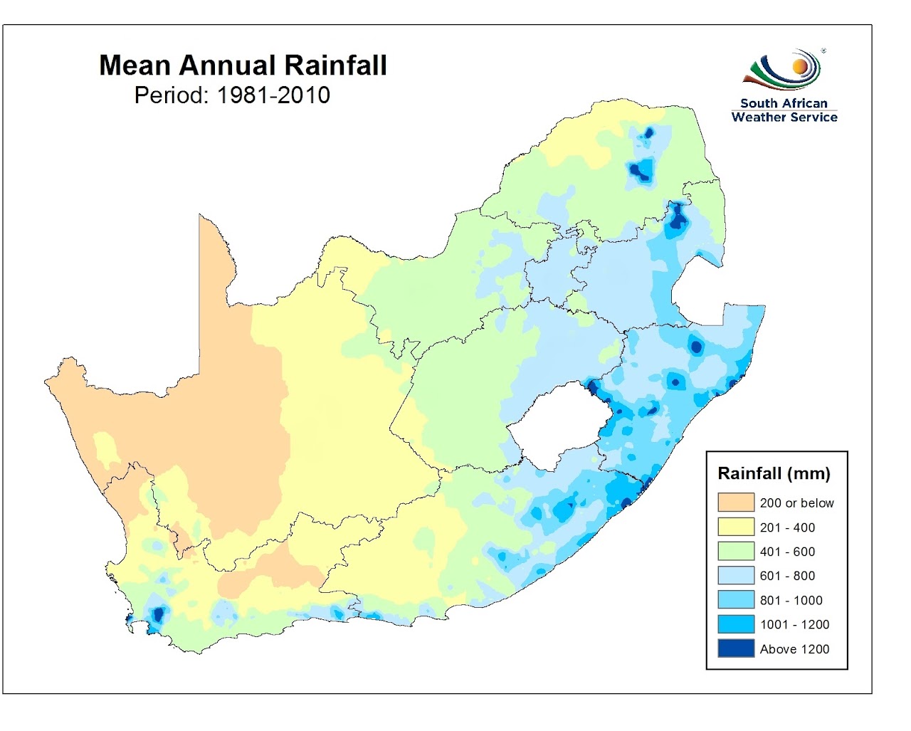
Geostatistical Data: Why interpolation?

Objective is to create a smoothed surface Assumptions: Surface is continuous and Spatial dependence Too expensive to sample exhaustively Physically impossible to get to locations Inaccessible locations e.t.c.

Areal (Lattice) Data

• In areal or lattice data, the domain is a fixed countable A. Observations are associated with regions:

\[ Z(A_i), i=1,\ldots,n \]

• Observations are made over the fixed set of spatial units (regular or irregular polygons)
• Data are typically aggregated at area level (e.g. districts, census tracts, grid cells)
• Units are non-overlapping
• Common in spatial epidemiology: cases aggregated by administrative area
• Useful for analysing spatial patterns and identifying geographic risk factors
• Spatial relationships (e.g. adjacency, neighborhood structure) are crucial
• Also arise in remote sensing where measurements are made on regular grids (e.g. satellite-derived temperature or vegetation indices)

Examples: - Number of deaths due to Septicaemia in the municipalities of South Africa - Presence or absence of an invasive plant species in square quadrats over a study area - Pixel values from remote sensing

Point Pattern Data

• In point patterns, the domain is random \(D\).

• Its index set gives the locations of random events of the spatial point pattern, and \(Z(s)\) may be equal to \(1 s ∈ D\) indicating occurrence of the event, or random, giving some additional information.

• Point patterns arise when the variable to be analysed corresponds to the location of events

• The main interest is in the locations (points) of all occurrences of some event:

• Earthquake epicentres

• Location of road accidents

• Locations of longleaf pines

• The points may also be “marked” (e.g. magnitude of earthquakes as a marker of size)

• The question of interest is whether the points exhibits complete spatial randomness, clustering, or regularity

Comparison

Feature	Geostatistical	Lattice	Point Pattern
Observation	Measurement	Region	Event
Location fixed?	Yes	Yes	Random
Goal	Prediction	Explain variation	Model occurrence
Example	Rainfall	Census	Crashes

Which Statistical Models?

Data type	Typical methods
Geostatistical	Variograms, Kriging, Gaussian Processes
Lattice	Moran’s I, LISA, SAR, SEM
Point Pattern	Quadrat analysis, K-function, Kernel Density

Throughout this course we will study all three.

Spatial Data Issues to Watch For

• Modifiable Areal Unit Problem (MAUP): Sensitivity of results to zonal aggregation.
• Ecological Fallacy: Inappropriate inference about individuals from aggregated spatial data.
• Spatial Scale Dependency: Results vary depending on the chosen geographic resolution.
• Boundary & Edge Effects: Distortions arising at the margins of observation window \(D\).

The Modifiable Areal Unit Problem (MAUP)

Two Components of MAUP

• Scale Effect: Statistical results change as data are aggregated to larger spatial units.
• Zone Effect: Statistical results change when the shape or orientation of spatial units is altered.

Analytical Impact

MAUP directly influences:

• Data aggregation
• Correlation coefficients
• Variance
• Spatial autocorrelation
• Statistical inference

1. Scale Effect (Aggregation)

As point or grid data are aggregated into progressively larger spatial units, the sample variance decreases, while the overall mean remains unchanged.

Resolution	Grid Units	Mean (\(\bar{x}\))	Variance (\(s^2\))
Fine Scale	\(4\times4\) (\(n=16\))	3.75	2.60
Medium Scale	\(4\times2\) (\(n=8\))	3.75	0.50
Coarse Scale	\(2\times2\) (\(n=4\))	3.75	0.00

\[ \bar{x} = \frac{1}{n} \sum_{i=1}^{n}x_i \]

\[ s^2 = \frac{1}{n-1} \sum_{i=1}^{n} (x_i-\bar{x})^2 \]

2. Zone Effect (Alternative Zoning)

Holding the number of spatial units constant, changing the shape or orientation of zones changes the calculated statistics.

Zoning Scheme	Layout	Mean (\(\bar{x}\))	Variance (\(s^2\))
Horizontal	\(2\times4\) (\(n=8\))	3.75	0.93
Vertical	\(4\times1\) (\(n=4\))	3.75	1.04
Irregular	\(n=4\)	3.17	2.11

library(sf)
library(dplyr)

# Define fine-scale grid data (Matrix a)
a_vals <- matrix(c(2,4,6,1,
                   3,4,3,5,
                   1,5,4,2,
                   5,4,5,4), nrow = 4, byrow = TRUE)

# Calculate original fine-scale statistics
cat("Original Grid (a): Mean =", mean(a_vals), "| Variance =", round(var(as.vector(a_vals)), 2), "\n")

Original Grid (a): Mean = 3.625 | Variance = 2.25 

# Aggregation (Matrix b - 2 columns per row average)
b_vals <- apply(a_vals, 1, function(row) c(mean(row[1:2]), mean(row[3:4])))
cat("Aggregated Grid (b): Mean =", mean(b_vals), "| Variance =", round(var(as.vector(b_vals)), 2), "\n")

Aggregated Grid (b): Mean = 3.625 | Variance = 0.41 

Key Message

Changing either the spatial scale or the zoning system can change the conclusions drawn from the same underlying data.

Exploratory Spatial Data Analysis (ESDA)

Prerequisites

You need to have the following R packages installed and recalled into your library:

suppressPackageStartupMessages({
library(sf)
library(spatstat)
library(spatstat.data)
library(ggplot2)
library(sp)
library(animation)
library(plotrix)
library(tmap)})

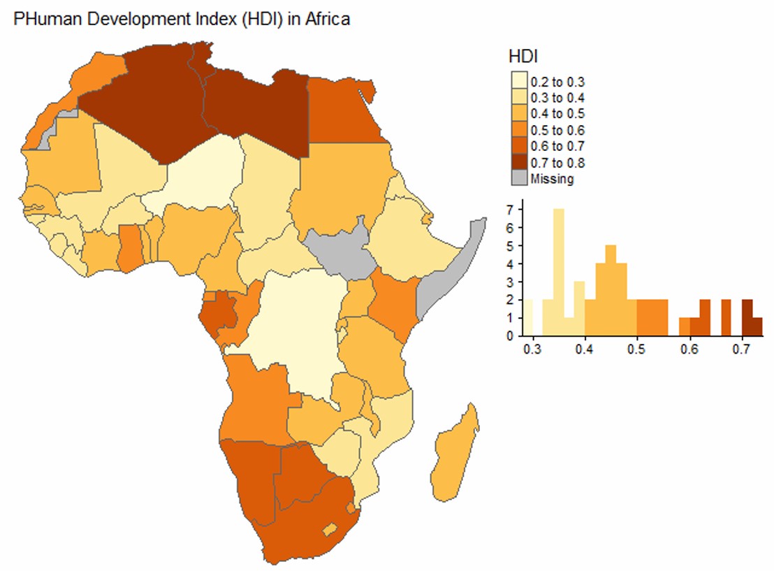
Datasets - Readily Available, Imported, Simulated Datasets

Simple Feature Basics

library(sf)

sf geometry types:

• point: st_point()
• linestring: st_linestring()
• polygon: st_polygon()
• multipoint: st_multipoint()
• multilinestring: st_multilinestring()
• multipolygon: st_multipolygon()
• collection of different geometry types: st_geometrycollection()

sfg

• A single point and multipoint

# Using the sf library for simple features

# Tarih      Saat      Enlem(N)  Boylam(E) Derinlik(km)  MD   ML   Mw    Yer                                             Çözüm Niteliği
# ---------- --------  --------  -------   ----------    ------------    --------------                                  --------------
# 2023.02.15 14:46:46  36.8803   36.6177        8.3      -.-  2.8  -.-   ASAGIBILENLER-ISLAHIYE (GAZIANTEP)                
# 2023.02.15 14:43:05  37.0218   28.8915        8.4      -.-  2.7  -.-   OTMANLAR-KOYCEGIZ (MUGLA)


# sf::st_crs(4326), which means x and y positions are interpreted as longitude (E) and latitude (N), respectively, in the World Geodetic System 1984 (WGS84)

point1_sg = c(36.6177, 36.8803) |> st_point() # this will create a "sfg" class Geometry
plot(point1_sg)

class(point1_sg)

[1] "XY"    "POINT" "sfg"  

point2_sg = c(28.8915, 37.0218) |> st_point()
plot(point2_sg)

class(point2_sg)

[1] "XY"    "POINT" "sfg"  

points_sg = rbind(c(36.6177, 36.8803),c(28.8915, 37.0218)) |> st_multipoint()
plot(points_sg)

class(points_sg)

[1] "XY"         "MULTIPOINT" "sfg"       

st_crs(points_sg)

Coordinate Reference System: NA

• A single polygon and a multipolygon

# polygon
poly1 = list(rbind(c(35.8337398, 37.8864154), 
                   c(36.3281246, 36.7682256),
                   c(38.5803218, 37.7562395), 
                   c(36.7346187, 38.5939762),
                   c(35.8337398, 37.8864154))) 

poly1_sg = poly1 |> st_polygon()

poly2 = list(rbind(c(36.7346187, 38.5939762), 
                   c(38.5913081, 39.3456266),
                   c(38.5803218, 37.7562395), 
                   c(36.7346187, 38.5939762)))

poly2_sg = poly2 |> st_polygon()

plot(poly1_sg)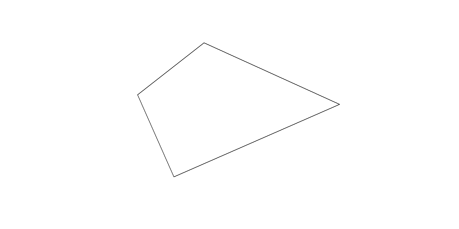

plot(poly2_sg)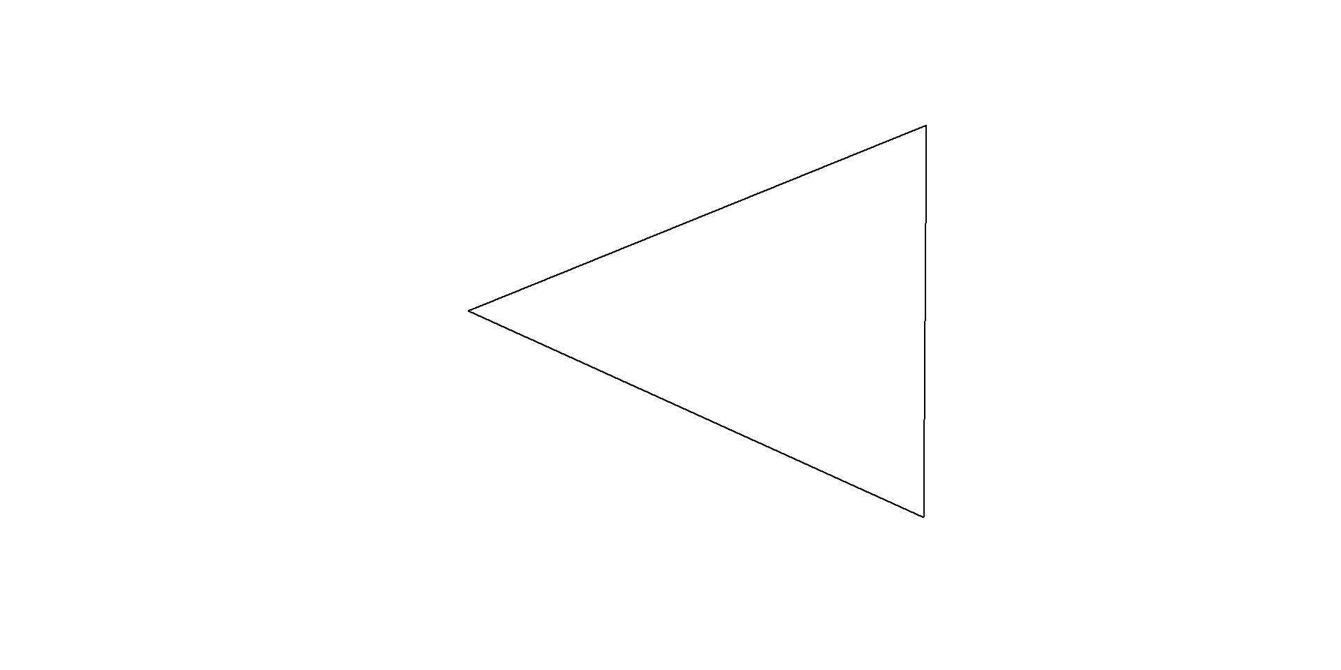

# multipolygon
polygons <- list(poly1, poly2)
polygons_sg <- polygons |> st_multipolygon()

st_crs(polygons_sg) # we see that the sf geometry has no CRS set up.

Coordinate Reference System: NA

sfc

• We usually work with multiple simple features and want to combine them. We have a multipolygon and points and want to combine these. We will use st_sfc() to merge

points_sfc <- st_sfc(point1_sg, point2_sg)                   # with no CRS
st_crs(points_sfc)

Coordinate Reference System: NA

points_sfc <- st_sfc(point1_sg, point2_sg, crs = 4326)       # with appropriate CRS
st_crs(points_sfc)

Coordinate Reference System:
  User input: EPSG:4326 
  wkt:
GEOGCRS["WGS 84",
    ENSEMBLE["World Geodetic System 1984 ensemble",
        MEMBER["World Geodetic System 1984 (Transit)"],
        MEMBER["World Geodetic System 1984 (G730)"],
        MEMBER["World Geodetic System 1984 (G873)"],
        MEMBER["World Geodetic System 1984 (G1150)"],
        MEMBER["World Geodetic System 1984 (G1674)"],
        MEMBER["World Geodetic System 1984 (G1762)"],
        MEMBER["World Geodetic System 1984 (G2139)"],
        MEMBER["World Geodetic System 1984 (G2296)"],
        ELLIPSOID["WGS 84",6378137,298.257223563,
            LENGTHUNIT["metre",1]],
        ENSEMBLEACCURACY[2.0]],
    PRIMEM["Greenwich",0,
        ANGLEUNIT["degree",0.0174532925199433]],
    CS[ellipsoidal,2],
        AXIS["geodetic latitude (Lat)",north,
            ORDER[1],
            ANGLEUNIT["degree",0.0174532925199433]],
        AXIS["geodetic longitude (Lon)",east,
            ORDER[2],
            ANGLEUNIT["degree",0.0174532925199433]],
    USAGE[
        SCOPE["Horizontal component of 3D system."],
        AREA["World."],
        BBOX[-90,-180,90,180]],
    ID["EPSG",4326]]

multipolygon_sfc <- st_sfc(poly1_sg, poly2_sg, crs = 4326)
st_crs(multipolygon_sfc)

Coordinate Reference System:
  User input: EPSG:4326 
  wkt:
GEOGCRS["WGS 84",
    ENSEMBLE["World Geodetic System 1984 ensemble",
        MEMBER["World Geodetic System 1984 (Transit)"],
        MEMBER["World Geodetic System 1984 (G730)"],
        MEMBER["World Geodetic System 1984 (G873)"],
        MEMBER["World Geodetic System 1984 (G1150)"],
        MEMBER["World Geodetic System 1984 (G1674)"],
        MEMBER["World Geodetic System 1984 (G1762)"],
        MEMBER["World Geodetic System 1984 (G2139)"],
        MEMBER["World Geodetic System 1984 (G2296)"],
        ELLIPSOID["WGS 84",6378137,298.257223563,
            LENGTHUNIT["metre",1]],
        ENSEMBLEACCURACY[2.0]],
    PRIMEM["Greenwich",0,
        ANGLEUNIT["degree",0.0174532925199433]],
    CS[ellipsoidal,2],
        AXIS["geodetic latitude (Lat)",north,
            ORDER[1],
            ANGLEUNIT["degree",0.0174532925199433]],
        AXIS["geodetic longitude (Lon)",east,
            ORDER[2],
            ANGLEUNIT["degree",0.0174532925199433]],
    USAGE[
        SCOPE["Horizontal component of 3D system."],
        AREA["World."],
        BBOX[-90,-180,90,180]],
    ID["EPSG",4326]]

sf

We usually have a data frame that stores the attributes of points, polygons, lines. Remember the earthquake magnitude, time, depth for the points; elevation, population, size for the polygons.

For points

magnitude = c(2.8, 2.7)
depth = c(8.3, 8.4)
time = c(1446, 1443)

earthquake_marks = data.frame(magnitude, depth, time)

earthquake_sf <- earthquake_marks |> st_sf(geometry = points_sfc)    # sf object

plot1 = ggplot() + 
  geom_sf(data = earthquake_sf["magnitude"], color = "black") +
  coord_sf() 
plot1

External files (csv, shp etc)

We will use two layers:

• Location of earthquakes - earthquakes
• Boundaries of Turkey as a polygon - turkeyshp

One of the files is a shp file, the other one is just a simple csv file.

• Location of earthquakes - earthquakes (from a csv)

Read in the dataset as usual

earthquake_csv <- read.csv("C:/Users/01438475/OneDrive - University of Cape Town/ASDA/DataSets/EarthquakesTR.csv")
head(earthquake_csv)

       Tarih     Saat     Lat    Long Derinlik_km  MD  ML  Mw
1 2023.02.07 13:44:51 38.2452 37.9093        13.9 -.- 3.5 -.-
2 2023.02.07 13:41:44 38.1057 36.5072         5.0 -.- 3.9 -.-
3 2023.02.07 13:37:24 36.4372 35.6998        13.4 -.- 4.0 -.-
4 2023.02.07 13:32:27 37.2445 36.9277         5.4 -.- 2.5 -.-
5 2023.02.07 13:30:10 38.1428 37.8203         2.0 -.- 2.9 -.-
6 2023.02.07 13:27:30 38.3478 38.1357         6.5 -.- 4.7 -.-
                               Yer
1           OREN-AKCADAG (MALATYA)
2 MAHMUTBEY-GOKSUN (KAHRAMANMARAS)
3     ISKENDERUN KORFEZI (AKDENIZ)
4      NAIMLER-NURDAGI (GAZIANTEP)
5   FINDIKKOY-DOGANSEHIR (MALATYA)
6     KUSDOGAN-YESILYURT (MALATYA)

earthquake_sf <- earthquake_csv |> 
  st_as_sf(coords = c("Long", "Lat"), crs = 4326)  |>      # convert to sf file |>
  #Here Long comes first.
  st_transform("+proj=utm +zone=37 +datum=WGS84 +units=m +no_defs")                                        # this could be a different CRS

st_crs(earthquake_sf)

Coordinate Reference System:
  User input: +proj=utm +zone=37 +datum=WGS84 +units=m +no_defs 
  wkt:
PROJCRS["unknown",
    BASEGEOGCRS["unknown",
        DATUM["World Geodetic System 1984",
            ELLIPSOID["WGS 84",6378137,298.257223563,
                LENGTHUNIT["metre",1]],
            ID["EPSG",6326]],
        PRIMEM["Greenwich",0,
            ANGLEUNIT["degree",0.0174532925199433],
            ID["EPSG",8901]]],
    CONVERSION["UTM zone 37N",
        METHOD["Transverse Mercator",
            ID["EPSG",9807]],
        PARAMETER["Latitude of natural origin",0,
            ANGLEUNIT["degree",0.0174532925199433],
            ID["EPSG",8801]],
        PARAMETER["Longitude of natural origin",39,
            ANGLEUNIT["degree",0.0174532925199433],
            ID["EPSG",8802]],
        PARAMETER["Scale factor at natural origin",0.9996,
            SCALEUNIT["unity",1],
            ID["EPSG",8805]],
        PARAMETER["False easting",500000,
            LENGTHUNIT["metre",1],
            ID["EPSG",8806]],
        PARAMETER["False northing",0,
            LENGTHUNIT["metre",1],
            ID["EPSG",8807]],
        ID["EPSG",16037]],
    CS[Cartesian,2],
        AXIS["(E)",east,
            ORDER[1],
            LENGTHUNIT["metre",1,
                ID["EPSG",9001]]],
        AXIS["(N)",north,
            ORDER[2],
            LENGTHUNIT["metre",1,
                ID["EPSG",9001]]]]

• Boundaries of Turkey as a polygon - turkeyshp

turkeyshp = "C:/Users/01438475/OneDrive - University of Cape Town/ASDA/DataSets/turkey_administrativelevels0_1_2/tur_polbnda_adm0.shp" |>
  st_read() |>
  st_transform("+proj=utm +zone=37 +datum=WGS84 +units=m +no_defs")

Reading layer `tur_polbnda_adm0' from data source 
  `C:\Users\01438475\OneDrive - University of Cape Town\ASDA\DataSets\turkey_administrativelevels0_1_2\tur_polbnda_adm0.shp' 
  using driver `ESRI Shapefile'
Simple feature collection with 1 feature and 5 fields
Geometry type: MULTIPOLYGON
Dimension:     XY
Bounding box:  xmin: 25.66851 ymin: 35.80842 xmax: 44.81793 ymax: 42.10479
Geodetic CRS:  WGS 84

Plotting the two together in a simple plot:

plot(st_geometry(turkeyshp))
plot(st_geometry(earthquake_sf), add = TRUE, col = "red")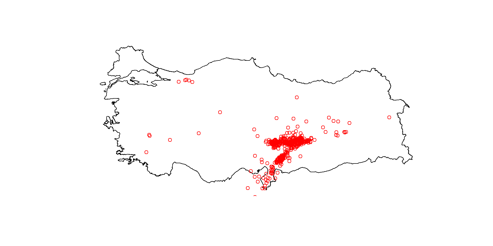

or using geom_sf() in ggplot:

plot1 = ggplot() +
  geom_sf(data = turkeyshp) +
  geom_sf(data = earthquake_sf) +
  theme_minimal()

Here you see that earthquakes outside of Turkey are also plotted. We can subset only the earthquakes that happened in Turkey:

earthquake_sf = earthquake_sf[turkeyshp,]
plot2 = ggplot() +
  geom_sf(data = turkeyshp) +
  geom_sf(data = earthquake_sf) +
  theme_minimal()

Visualisations can be done via tmap package as well, and can be saved as png, html files.

tmap_mode("view")
tmap1 = tm_shape(turkeyshp)+tm_polygons() +tm_shape(earthquake_sf) + tm_dots()
tmap_save(tmap1, filename= "turkeyearthquakes.html")

Simulated Datasets

CSR Data Points

set.seed(135)
xy_csr <- matrix(runif(80), ncol=2)
pp_csr <- as.ppp(xy_csr, c(0,1,0,1))
plot(pp_csr)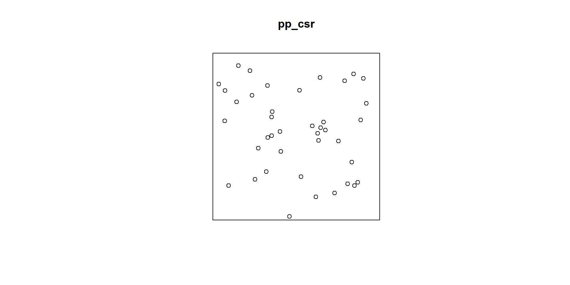

CSR Data Points with Marks

set.seed(135)
xy_csr <- matrix(runif(2000), ncol=2)
mark_numerical = rexp(1000)
mark_categorical =  sample(0:1,size=1000,replace=TRUE)

# plot without marks
pp_csr_m <- as.ppp(xy_csr, c(0,1,0,1))
plot(pp_csr_m)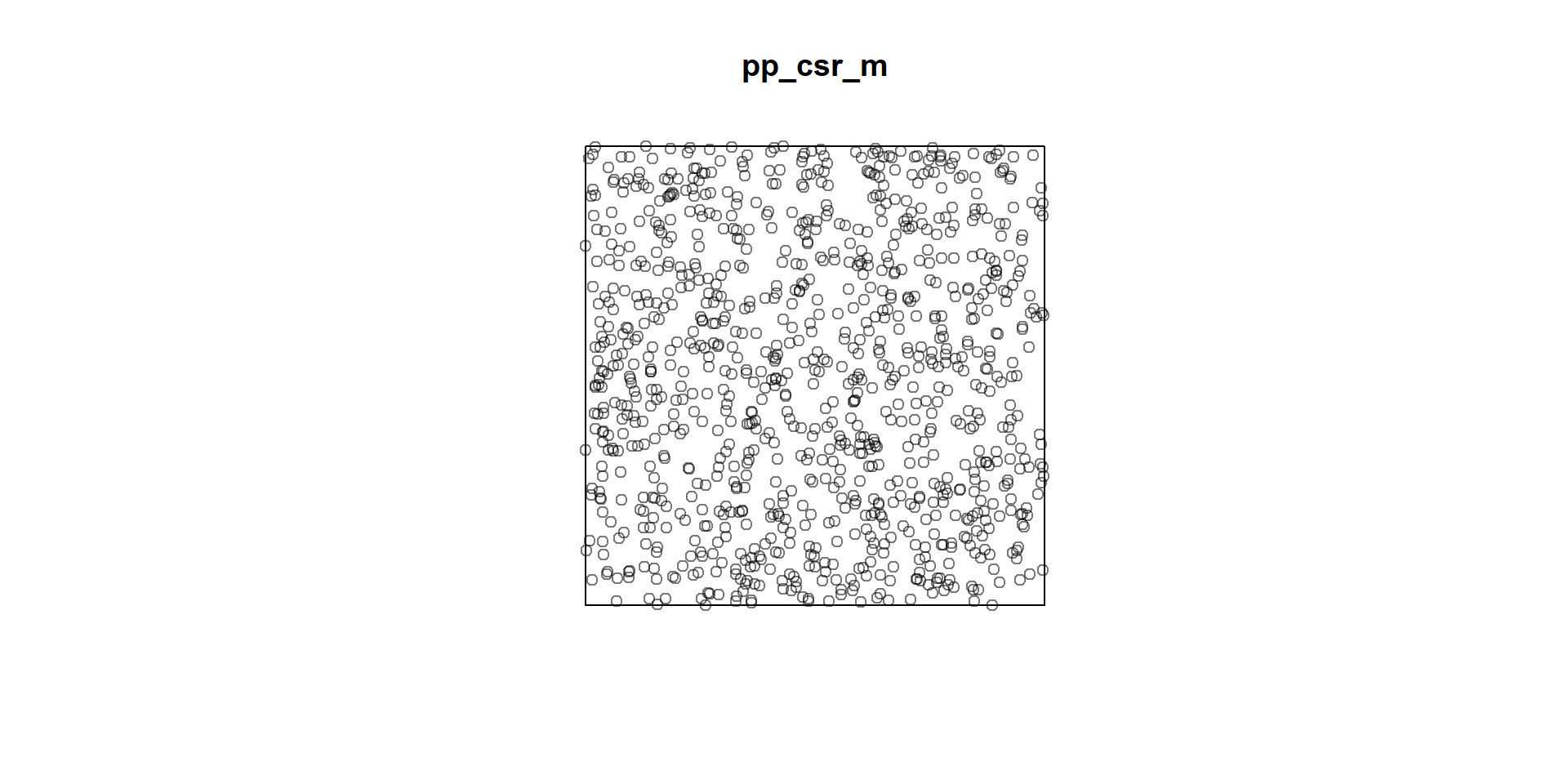

# plot with marks
xy_csr_withmark = as.data.frame(cbind(xy_csr,mark_numerical, mark_categorical))

# The categorical variable needs to be set as factor with clearly defined levels

xy_csr_withmark$mark_categorical = factor(xy_csr_withmark$mark_categorical, levels = c("0","1"))

# set as point pattern

pp_csr_withmark = with(xy_csr_withmark, ppp(V1,V2,c(0,1),c(0,1),marks=xy_csr_withmark[,4]))
plot(pp_csr_withmark)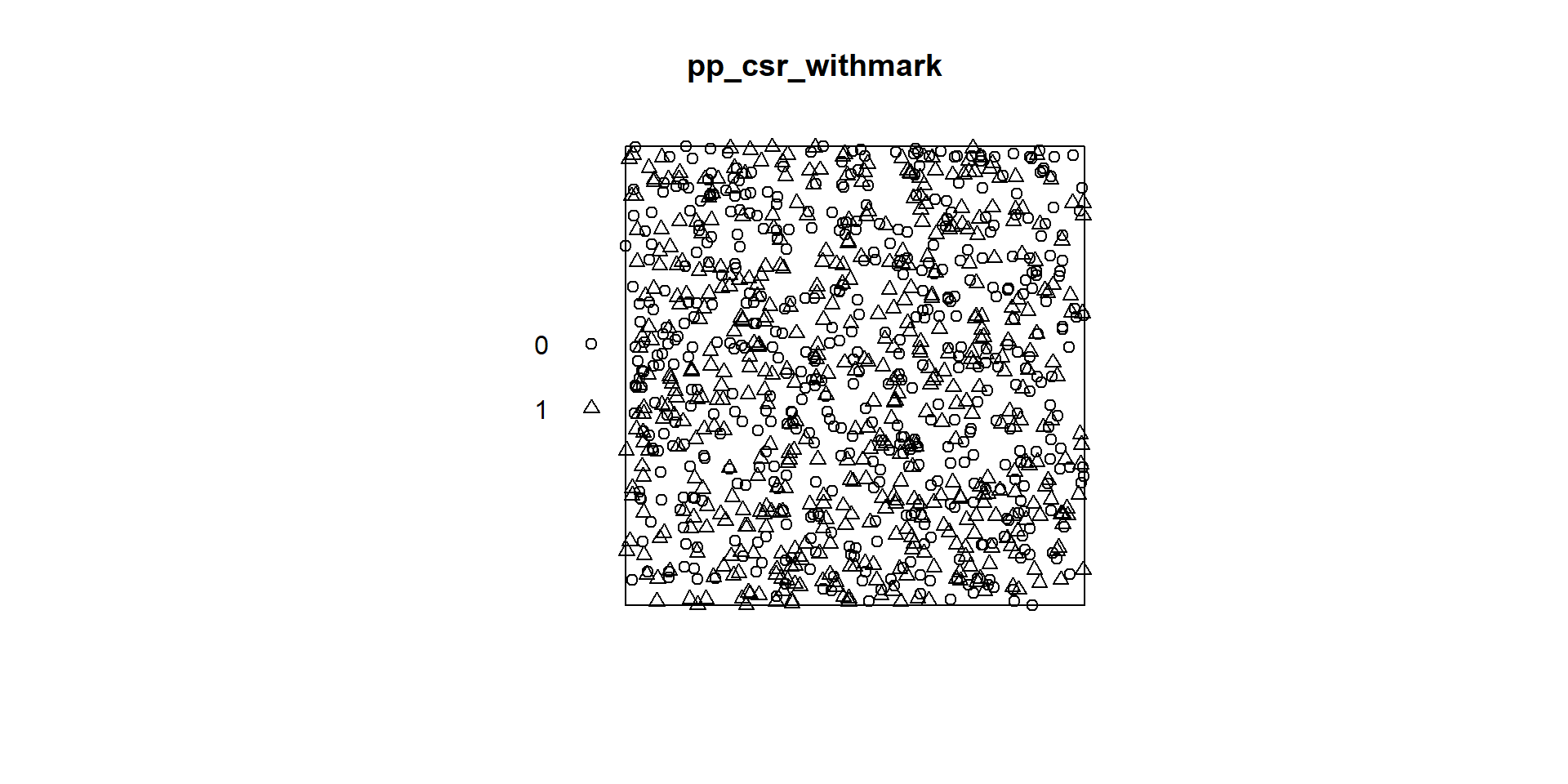

Regular Data Points

regular <- read.csv("C:/Users/01438475/OneDrive - University of Cape Town/ASDA/regular.csv")
xy_regular <- matrix(cbind(regular$X,regular$Y), ncol=2)
pp_regular <- as.ppp(xy_regular, c(0,1,0,1))
plot(pp_regular)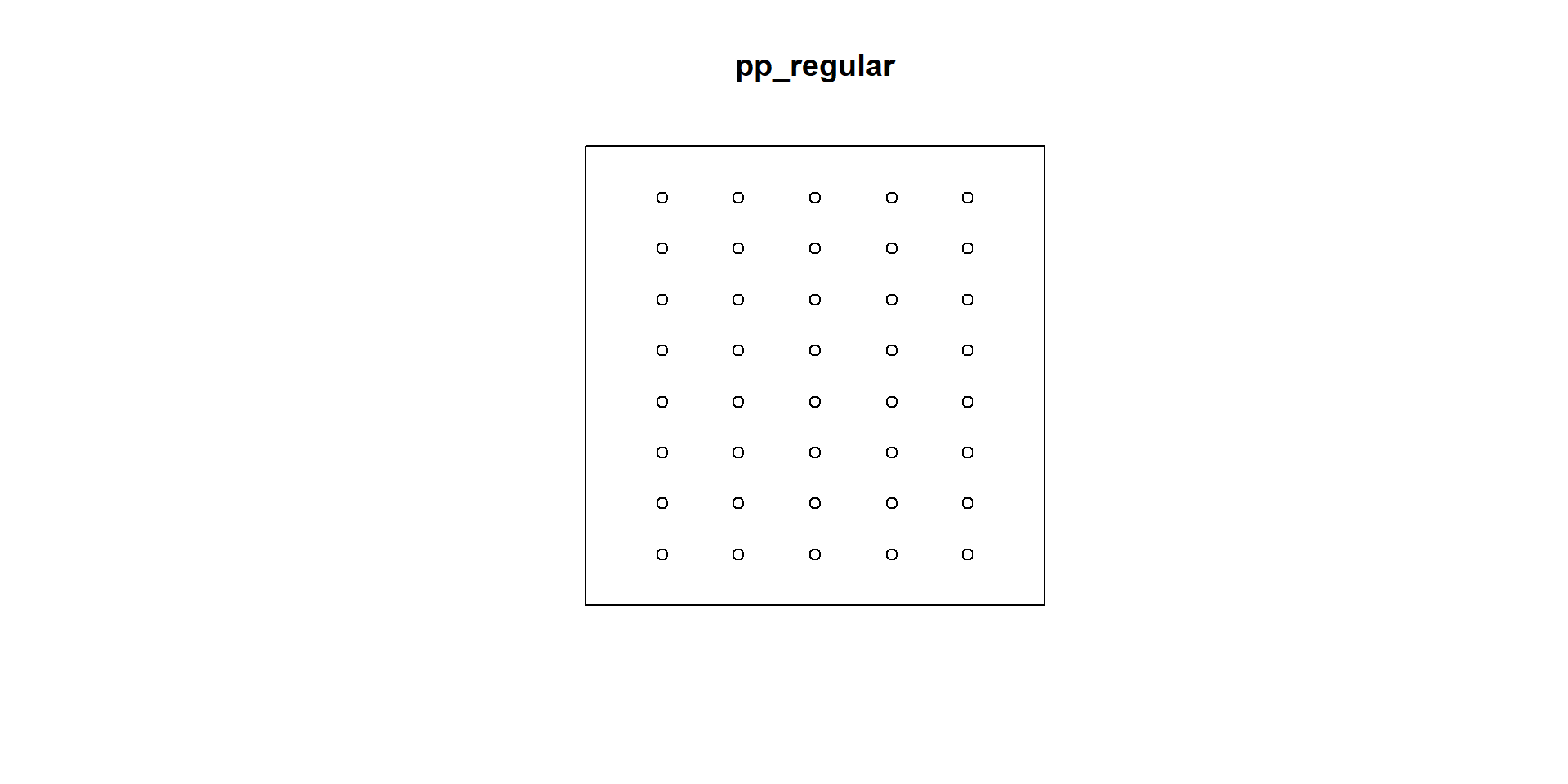

Cluster Data Points

cluster <- read.csv("C:/Users/01438475/OneDrive - University of Cape Town/ASDA/cluster.csv")
xy_cluster <- matrix(cbind(cluster$X,cluster$Y), ncol=2)
pp_cluster <- as.ppp(xy_cluster, c(0,1,0,1))
plot(pp_cluster)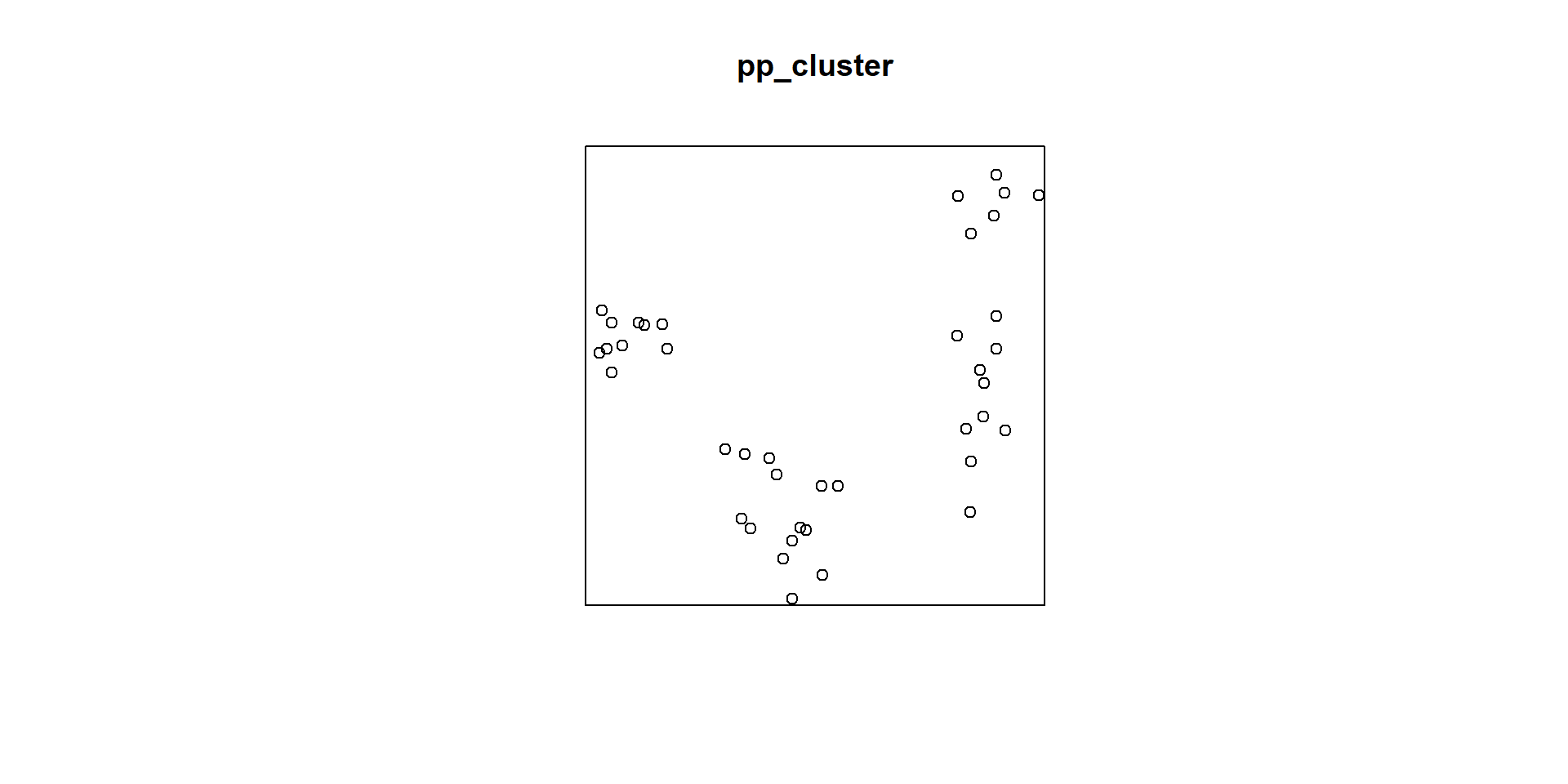

Swedishpines Dataset from spatstat.data library

data(swedishpines)
swp = rescale.ppp(swedishpines)
swp

Planar point pattern: 71 points
window: rectangle = [0, 9.6] x [0, 10] metres

class(swp)

[1] "ppp"

summary(swp)

Planar point pattern:  71 points
Average intensity 0.7395833 points per square metre

Coordinates are given to 16 decimal places

Window: rectangle = [0, 9.6] x [0, 10] metres
Window area = 96 square metres
Unit of length: 1 metre

plot(swp)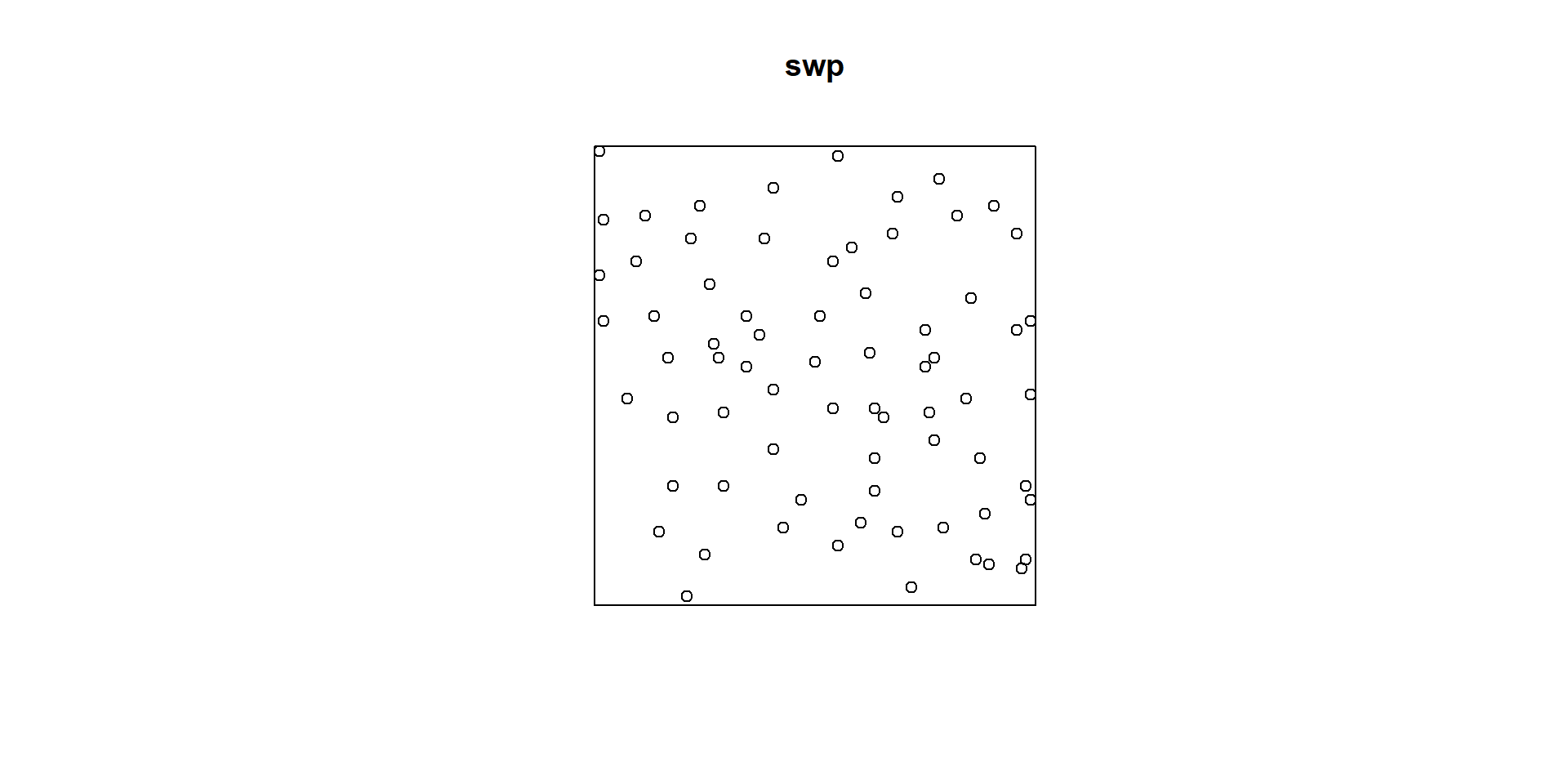

Tesselation

Given n distinct events xi in a planar region A, we can assign to xi a “territory” consisting of that part of A which is closer to xi than to any other xj. This construction, referred to either as the Dirichlet tessellation or Voronoi tessellation of the events in A, has been incorporated into stochastic models of natural phenomena such as inter-plant competition

Events xi and xj whose cells share a common boundary segment are said to be contiguous. Typically, each cell vertex is common to three cells, and the lines joining the pairs of contiguous events define a triangulation of the xi, called the Delaunay triangulation. Thus, cell boundaries can be obtained as the perpendicular bisectors of the edges of the triangulation, and cell vertices are the corresponding circumcentres

# convert the swp into sf
swp_sf_pp = st_as_sf(swp)
class(swp_sf_pp)

[1] "sf"         "data.frame"

st_crs(swp_sf_pp)

Coordinate Reference System: NA

# Run deldir on point coordinates
dd <- deldir(swp$x, swp$y)

# create tiles around
tiles <- tile.list(dd)
tile_to_polygon <- function(tile) {
  coords <- cbind(tile$x, tile$y)
  coords <- rbind(coords, coords[1,])
  st_polygon(list(coords))
}

polys <- lapply(tiles, tile_to_polygon)
sf_tiles <- st_sf(
  id = sapply(tiles, function(t) t$ptNum),
  geometry = st_sfc(polys)
)
ggplot() +
  geom_sf(data = swp_sf_pp, color = "red", size = 2) + geom_sf(data = sf_tiles, fill = NA, color = "black") +
  theme_minimal() +
  labs(title = "Dirichlet (Voronoi) Tessellation with sf")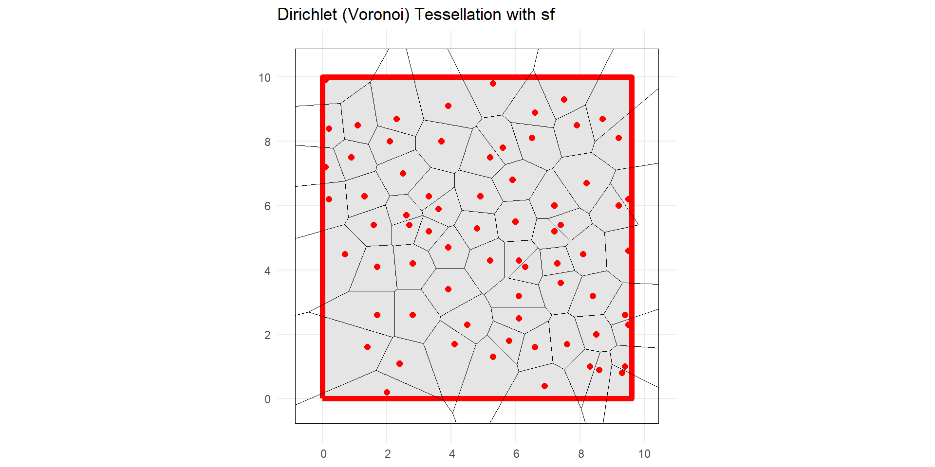

External datasets - Turkey

Let us go back to Earthquake data that we converted to sf object.

Convert the sf objects to ppp point pattern object using function as.ppp so that we can analyse them in R with spatstat.

# only the geometry
earthquake_ppp = as.ppp(st_geometry(earthquake_sf))
turkeyshp_owin = as.owin(st_geometry(turkeyshp))

plot(earthquake_ppp)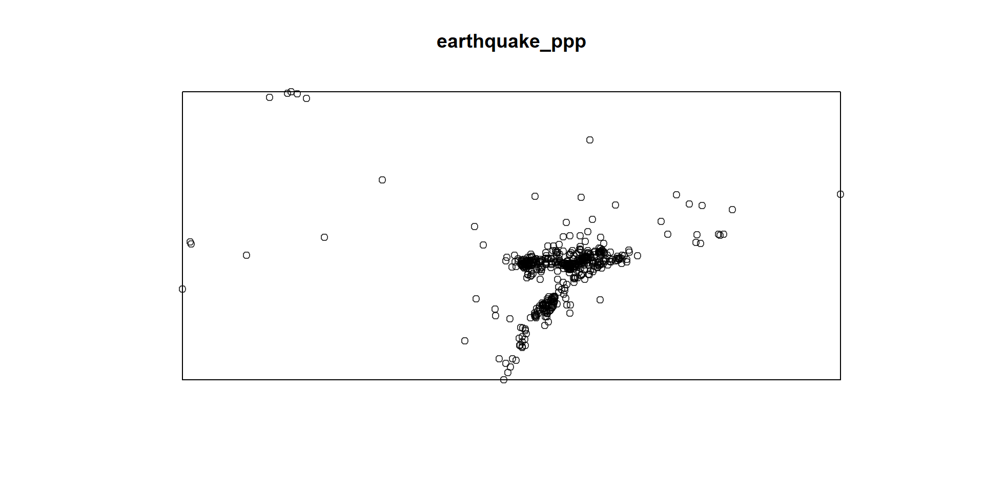

plot(turkeyshp_owin)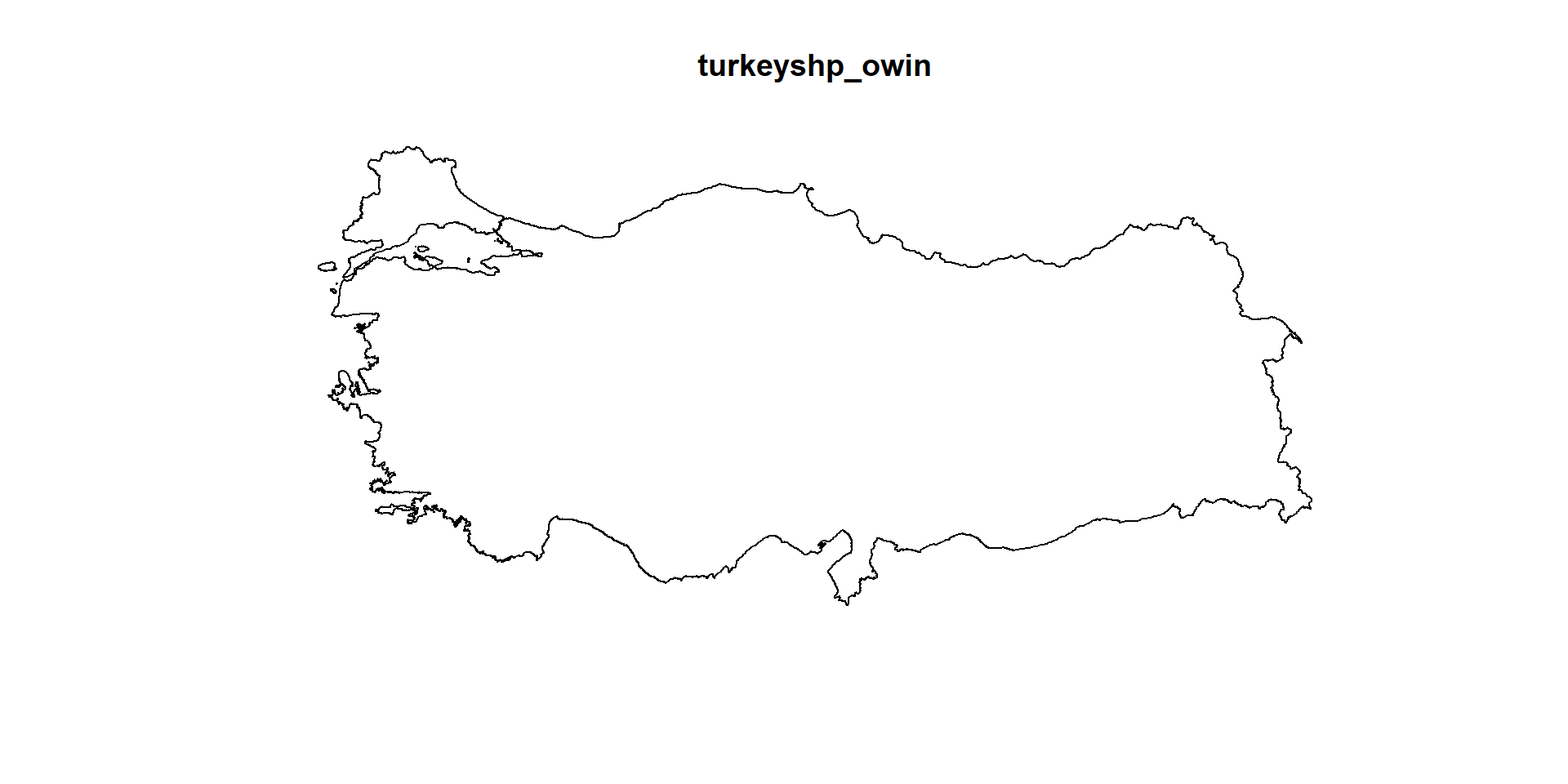

The observation window and the point pattern can be combined, so that the custom window replaces the default rectangular window:

earthquake_ppp = earthquake_ppp[turkeyshp_owin]
plot(earthquake_ppp)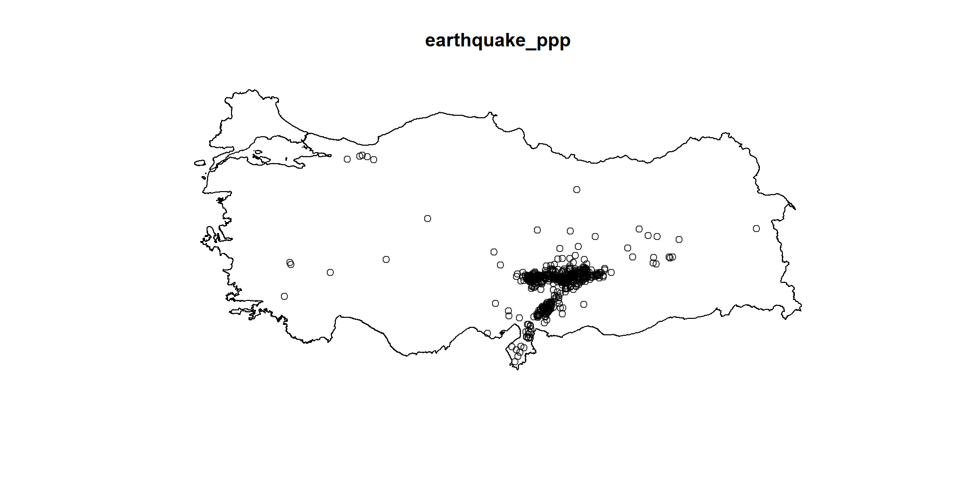

We might want to incorporate some marks to these points:

# if there are marks that need to be included:

earthquake_ppp.marked_numeric <- ppp(earthquake_ppp$x, earthquake_ppp$y, window = turkeyshp_owin, marks =data.frame(earthquake_sf)$ML)

plot(earthquake_ppp.marked_numeric, use.marks=TRUE)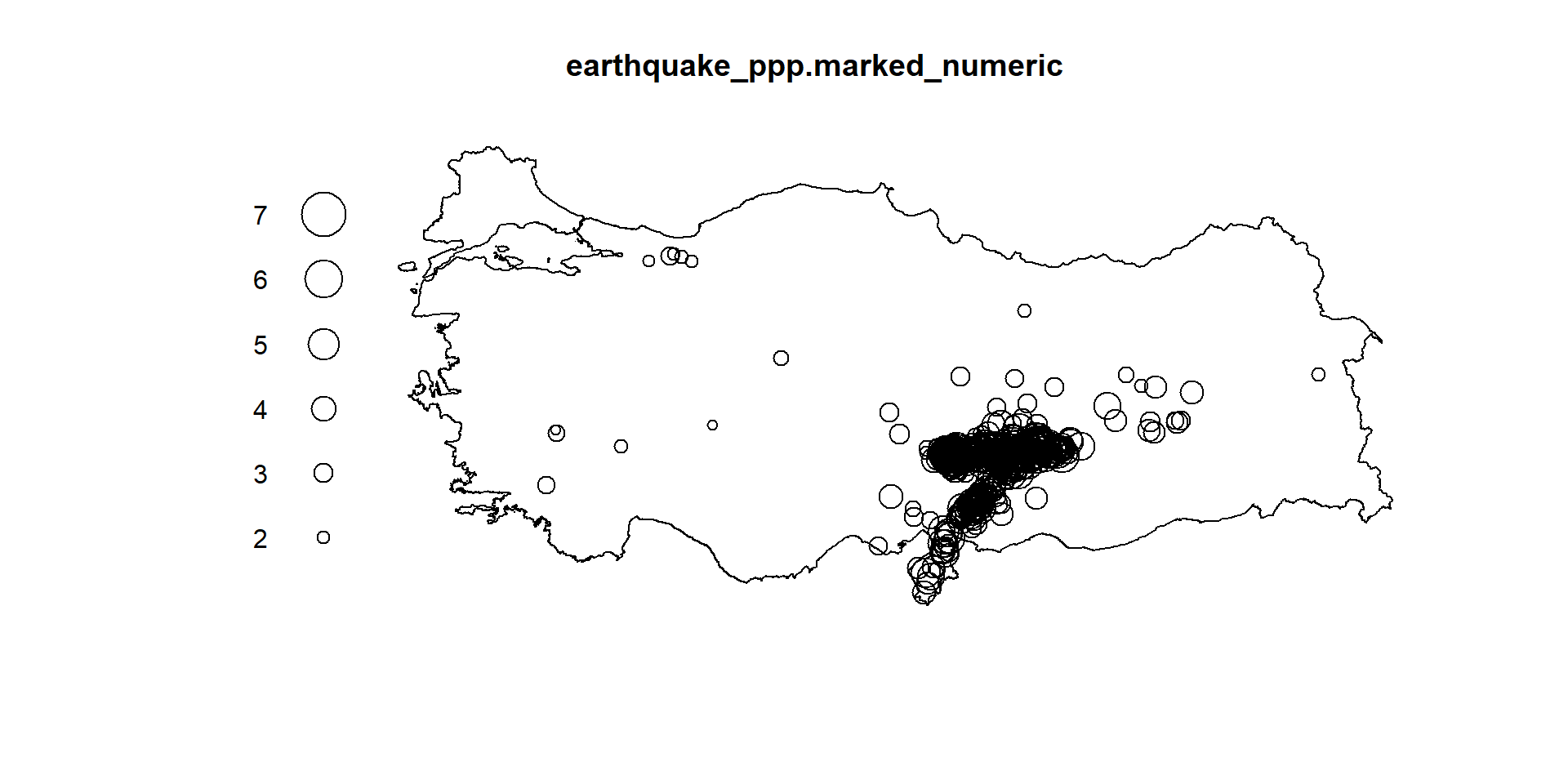

earthquake_ppp.marked_categorical <- ppp(earthquake_ppp$x, earthquake_ppp$y, window = turkeyshp_owin, marks =ifelse(data.frame(earthquake_sf)$ML<5,"low","high"))

plot(earthquake_ppp.marked_categorical, use.marks=TRUE, 
     cols=c("red","blue","pink"),
     markscale=0.1,
     pch=21, cex=1)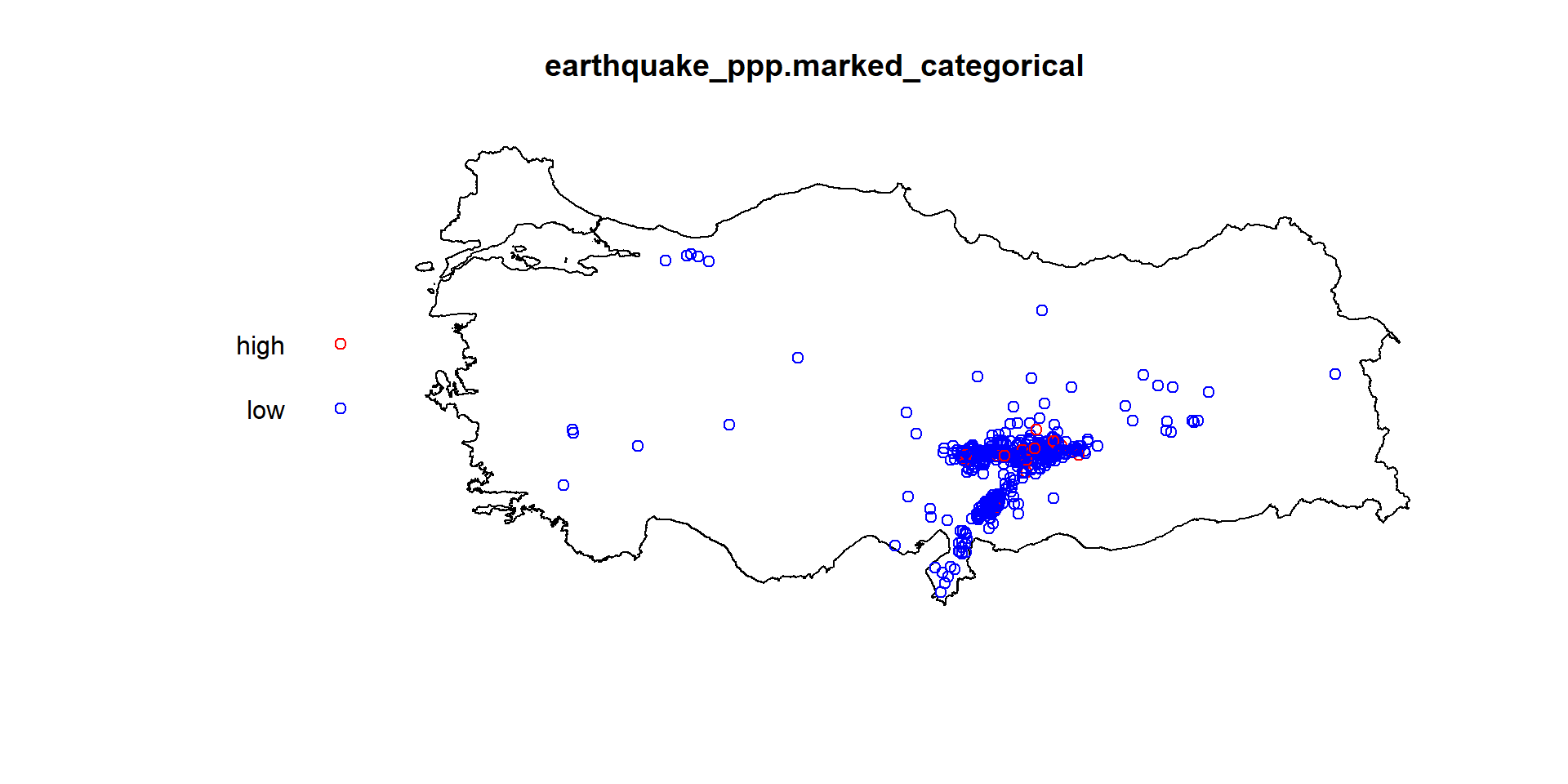

https://rspatial.org/raster/rosu/Chapter5.html https://geobgu.xyz/r/point-pattern-analysis.html https://www.keene.edu/campus/maps/tool/ https://data.humdata.org/dataset/cod-ab-tur? https://www.jla-data.net/eng/merging-geometry-of-sf-objects-in-r/

External Datasets - Clinics Dataset SA

Download the data from the following:

https://web1.capetown.gov.za/web1/OpenDataPortal/DatasetDetail?DatasetName=Clinics

library(sf)

RSA_roads = "C:/Users/01438475/OneDrive - University of Cape Town/ASDA/DataSets/zafrds8ff5a/ZAF_roads.shp" |> 
  st_read() |> st_transform(4326)

Reading layer `ZAF_roads' from data source 
  `C:\Users\01438475\OneDrive - University of Cape Town\ASDA\DataSets\zafrds8ff5a\ZAF_roads.shp' 
  using driver `ESRI Shapefile'
Simple feature collection with 5559 features and 5 fields
Geometry type: MULTILINESTRING
Dimension:     XY
Bounding box:  xmin: 16.48784 ymin: -34.82747 xmax: 32.85267 ymax: -22.17693
Geodetic CRS:  WGS 84

RSA_biome = "C:/Users/01438475/OneDrive - University of Cape Town/ASDA/DataSets/rsabiome4xkhi/RSA_biome.shp" |> 
  st_read() |> st_transform(4326)

Reading layer `RSA_biome' from data source 
  `C:\Users\01438475\OneDrive - University of Cape Town\ASDA\DataSets\rsabiome4xkhi\RSA_biome.shp' 
  using driver `ESRI Shapefile'
Simple feature collection with 3127 features and 1 field
Geometry type: POLYGON
Dimension:     XY
Bounding box:  xmin: 16.45296 ymin: -34.8336 xmax: 32.8928 ymax: -22.12583
Geodetic CRS:  Hartebeesthoek94

clinics_sf = "C:/Users/01438475/OneDrive - University of Cape Town/ASDA/DataSets/Clinics/SL_CLNC.shp" |> 
  st_read() |> st_transform(4326)

Reading layer `SL_CLNC' from data source 
  `C:\Users\01438475\OneDrive - University of Cape Town\ASDA\DataSets\Clinics\SL_CLNC.shp' 
  using driver `ESRI Shapefile'
Simple feature collection with 149 features and 5 fields
Geometry type: POINT
Dimension:     XY
Bounding box:  xmin: 18.34268 ymin: -34.19491 xmax: 18.90847 ymax: -33.51262
Geodetic CRS:  WGS 84

ct.wards_sf <- "C:/Users/01438475/OneDrive - University of Cape Town/ASDA/DataSets/sa/CPT/electoral wards for cpt.shp" |>
  st_read(quiet = TRUE) |> 
  st_set_crs(4326)

st_crs(ct.wards_sf)

Coordinate Reference System:
  User input: EPSG:4326 
  wkt:
GEOGCRS["WGS 84",
    ENSEMBLE["World Geodetic System 1984 ensemble",
        MEMBER["World Geodetic System 1984 (Transit)"],
        MEMBER["World Geodetic System 1984 (G730)"],
        MEMBER["World Geodetic System 1984 (G873)"],
        MEMBER["World Geodetic System 1984 (G1150)"],
        MEMBER["World Geodetic System 1984 (G1674)"],
        MEMBER["World Geodetic System 1984 (G1762)"],
        MEMBER["World Geodetic System 1984 (G2139)"],
        MEMBER["World Geodetic System 1984 (G2296)"],
        ELLIPSOID["WGS 84",6378137,298.257223563,
            LENGTHUNIT["metre",1]],
        ENSEMBLEACCURACY[2.0]],
    PRIMEM["Greenwich",0,
        ANGLEUNIT["degree",0.0174532925199433]],
    CS[ellipsoidal,2],
        AXIS["geodetic latitude (Lat)",north,
            ORDER[1],
            ANGLEUNIT["degree",0.0174532925199433]],
        AXIS["geodetic longitude (Lon)",east,
            ORDER[2],
            ANGLEUNIT["degree",0.0174532925199433]],
    USAGE[
        SCOPE["Horizontal component of 3D system."],
        AREA["World."],
        BBOX[-90,-180,90,180]],
    ID["EPSG",4326]]

st_crs(clinics_sf)

Coordinate Reference System:
  User input: EPSG:4326 
  wkt:
GEOGCRS["WGS 84",
    ENSEMBLE["World Geodetic System 1984 ensemble",
        MEMBER["World Geodetic System 1984 (Transit)"],
        MEMBER["World Geodetic System 1984 (G730)"],
        MEMBER["World Geodetic System 1984 (G873)"],
        MEMBER["World Geodetic System 1984 (G1150)"],
        MEMBER["World Geodetic System 1984 (G1674)"],
        MEMBER["World Geodetic System 1984 (G1762)"],
        MEMBER["World Geodetic System 1984 (G2139)"],
        MEMBER["World Geodetic System 1984 (G2296)"],
        ELLIPSOID["WGS 84",6378137,298.257223563,
            LENGTHUNIT["metre",1]],
        ENSEMBLEACCURACY[2.0]],
    PRIMEM["Greenwich",0,
        ANGLEUNIT["degree",0.0174532925199433]],
    CS[ellipsoidal,2],
        AXIS["geodetic latitude (Lat)",north,
            ORDER[1],
            ANGLEUNIT["degree",0.0174532925199433]],
        AXIS["geodetic longitude (Lon)",east,
            ORDER[2],
            ANGLEUNIT["degree",0.0174532925199433]],
    USAGE[
        SCOPE["Horizontal component of 3D system."],
        AREA["World."],
        BBOX[-90,-180,90,180]],
    ID["EPSG",4326]]

class(clinics_sf)

[1] "sf"         "data.frame"

summary(clinics_sf)

     LCTN               ATHY               NAME              CLASS          
 Length:149         Length:149         Length:149         Length:149        
 Class :character   Class :character   Class :character   Class :character  
 Mode  :character   Mode  :character   Mode  :character   Mode  :character  
     RGN                     geometry  
 Length:149         POINT        :149  
 Class :character   epsg:4326    :  0  
 Mode  :character   +proj=long...:  0  

Swedishpines Dataset from spatstat.data library

data(swedishpines)
swp = rescale.ppp(swedishpines)
class(swp)

[1] "ppp"

summary(swp)

Planar point pattern:  71 points
Average intensity 0.7395833 points per square metre

Coordinates are given to 16 decimal places

Window: rectangle = [0, 9.6] x [0, 10] metres
Window area = 96 square metres
Unit of length: 1 metre

plot(swp)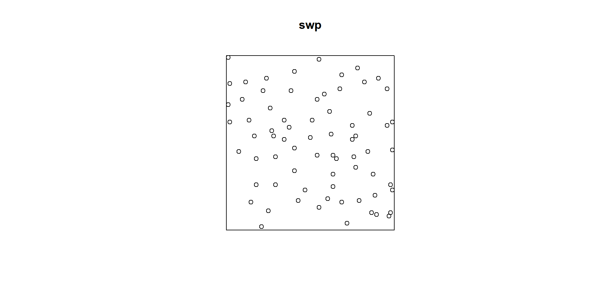

Clinics Dataset Using Simple Features (SF)

Download the data from the following:

https://web1.capetown.gov.za/web1/OpenDataPortal/DatasetDetail?DatasetName=Clinics

Extract the data frame into R:

library(sf)
clinics_sf = st_read("C:/Users/01438475/OneDrive - University of Cape Town/ASDA/DataSets/Clinics/SL_CLNC.shp")

Reading layer `SL_CLNC' from data source 
  `C:\Users\01438475\OneDrive - University of Cape Town\ASDA\DataSets\Clinics\SL_CLNC.shp' 
  using driver `ESRI Shapefile'
Simple feature collection with 149 features and 5 fields
Geometry type: POINT
Dimension:     XY
Bounding box:  xmin: 18.34268 ymin: -34.19491 xmax: 18.90847 ymax: -33.51262
Geodetic CRS:  WGS 84

clinics_sf

Simple feature collection with 149 features and 5 fields
Geometry type: POINT
Dimension:     XY
Bounding box:  xmin: 18.34268 ymin: -34.19491 xmax: 18.90847 ymax: -33.51262
Geodetic CRS:  WGS 84
First 10 features:
                                       LCTN              ATHY
1           C/O Adam/ Liedeman Street Mamre              PAWC
2                 Cnr Hermes & GrosvenorAve CITY OF CAPE TOWN
3            Hassen Kahn Ave Rusthof Strand              PAWC
4              61 Central Circle, Fish Hoek CITY OF CAPE TOWN
5                     Simon Street, Nomzamo CITY OF CAPE TOWN
6  C/O Musical and Hospital Street Macassar              PAWC
7            28 Church Street Somerset West CITY OF CAPE TOWN
8                       Fagan Street Strand CITY OF CAPE TOWN
9    Karbonkel Road, CMC Building, Hout Bay              PAWC
10                Midmar Street Groenvallei CITY OF CAPE TOWN
                     NAME                CLASS       RGN
1               MAMRE CDC Community Day Centre   Western
2        SAXON SEA CLINIC               Clinic   Western
3            GUSTROUW CDC Community Day Centre   Eastern
4        FISH HOEK CLINIC               Clinic  Southern
5              IKWEZI CDC Community Day Centre   Eastern
6            MACASSAR CDC Community Day Centre   Eastern
7    SOMERSET WEST CLINIC               Clinic   Eastern
8  FAGAN STREET SATELLITE            Satellite   Eastern
9    HOUT BAY HARBOUR CDC Community Day Centre  Southern
10  GROENVALLEI SATELLITE            Satellite Tygerberg
                     geometry
1  POINT (18.47692 -33.51262)
2  POINT (18.48881 -33.55012)
3  POINT (18.85211 -34.13472)
4  POINT (18.42632 -34.13669)
5  POINT (18.86622 -34.11375)
6  POINT (18.76369 -34.06105)
7  POINT (18.84814 -34.08579)
8   POINT (18.82979 -34.1162)
9   POINT (18.34268 -34.0549)
10 POINT (18.66701 -33.89165)

class(clinics_sf)

[1] "sf"         "data.frame"

summary(clinics_sf)

     LCTN               ATHY               NAME              CLASS          
 Length:149         Length:149         Length:149         Length:149        
 Class :character   Class :character   Class :character   Class :character  
 Mode  :character   Mode  :character   Mode  :character   Mode  :character  
     RGN                     geometry  
 Length:149         POINT        :149  
 Class :character   epsg:4326    :  0  
 Mode  :character   +proj=long...:  0  

Plotting Datasets

Basic plot() function

plot(swp)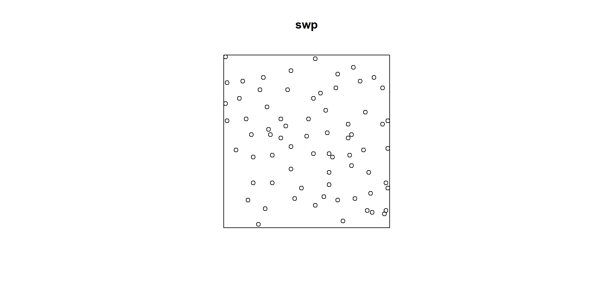

Basic ggplot() function - (sf) object

library(ggplot2)
plot1 = ggplot() + 
  geom_sf(data = clinics_sf, size = .8, color = "black") + 
  ggtitle("Location of Cape Town clinics - 2016") + 
  # not specifying crs here, coord_sf will use the CRS defined in the first layer = "+proj=longlat +datum=WGS84 +no_defs"
  coord_sf() 
plot1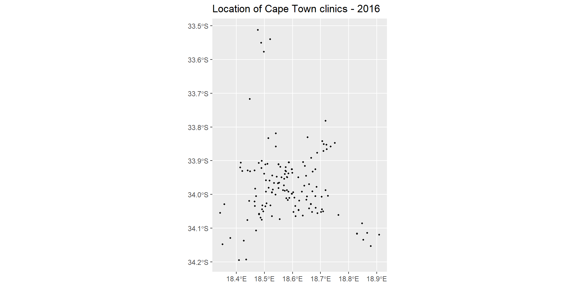

ggplot() function with a bounding box - (sf) object

library(ggplot2)
plot2 = ggplot() + 
  geom_sf(data = clinics_sf, size = .8, color = "black") + 
  ggtitle("Location of Cape Town clinics - 2016") + 
  coord_sf(xlim = c(18.34, 18.91), ylim = c(-34.19, -33.51262)) +
  theme(panel.grid.major = element_blank(), 
        panel.grid.minor = element_blank(),
        panel.background = element_rect(colour = "black", size=1, fill=NA))
plot2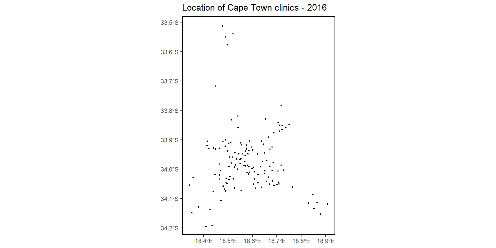

ggplot() with Electoral Wards Shape File

In order to plot using the electoral wards polygons, we need the sf data frame to be converted into Spatial Points Data Frame (sp).

clinics_sp <- as(clinics_sf, Class = "Spatial")
class(clinics_sp)

[1] "SpatialPointsDataFrame"
attr(,"package")
[1] "sp"

Download the CPT electoral wards and import the shape file as follows:

library(sf)
ct.wards_sf = st_read("C:/Users/01438475/OneDrive - University of Cape Town/ASDA/DataSets/sa/CPT/electoral wards for cpt.shp")

Reading layer `electoral wards for cpt' from data source 
  `C:\Users\01438475\OneDrive - University of Cape Town\ASDA\DataSets\sa\CPT\electoral wards for cpt.shp' 
  using driver `ESRI Shapefile'
Simple feature collection with 111 features and 9 fields
Geometry type: MULTIPOLYGON
Dimension:     XY
Bounding box:  xmin: 18.30722 ymin: -34.35834 xmax: 19.00467 ymax: -33.47128
CRS:           NA

st_geometry_type(ct.wards_sf)

  [1] MULTIPOLYGON MULTIPOLYGON MULTIPOLYGON MULTIPOLYGON MULTIPOLYGON
  [6] MULTIPOLYGON MULTIPOLYGON MULTIPOLYGON MULTIPOLYGON MULTIPOLYGON
 [11] MULTIPOLYGON MULTIPOLYGON MULTIPOLYGON MULTIPOLYGON MULTIPOLYGON
 [16] MULTIPOLYGON MULTIPOLYGON MULTIPOLYGON MULTIPOLYGON MULTIPOLYGON
 [21] MULTIPOLYGON MULTIPOLYGON MULTIPOLYGON MULTIPOLYGON MULTIPOLYGON
 [26] MULTIPOLYGON MULTIPOLYGON MULTIPOLYGON MULTIPOLYGON MULTIPOLYGON
 [31] MULTIPOLYGON MULTIPOLYGON MULTIPOLYGON MULTIPOLYGON MULTIPOLYGON
 [36] MULTIPOLYGON MULTIPOLYGON MULTIPOLYGON MULTIPOLYGON MULTIPOLYGON
 [41] MULTIPOLYGON MULTIPOLYGON MULTIPOLYGON MULTIPOLYGON MULTIPOLYGON
 [46] MULTIPOLYGON MULTIPOLYGON MULTIPOLYGON MULTIPOLYGON MULTIPOLYGON
 [51] MULTIPOLYGON MULTIPOLYGON MULTIPOLYGON MULTIPOLYGON MULTIPOLYGON
 [56] MULTIPOLYGON MULTIPOLYGON MULTIPOLYGON MULTIPOLYGON MULTIPOLYGON
 [61] MULTIPOLYGON MULTIPOLYGON MULTIPOLYGON MULTIPOLYGON MULTIPOLYGON
 [66] MULTIPOLYGON MULTIPOLYGON MULTIPOLYGON MULTIPOLYGON MULTIPOLYGON
 [71] MULTIPOLYGON MULTIPOLYGON MULTIPOLYGON MULTIPOLYGON MULTIPOLYGON
 [76] MULTIPOLYGON MULTIPOLYGON MULTIPOLYGON MULTIPOLYGON MULTIPOLYGON
 [81] MULTIPOLYGON MULTIPOLYGON MULTIPOLYGON MULTIPOLYGON MULTIPOLYGON
 [86] MULTIPOLYGON MULTIPOLYGON MULTIPOLYGON MULTIPOLYGON MULTIPOLYGON
 [91] MULTIPOLYGON MULTIPOLYGON MULTIPOLYGON MULTIPOLYGON MULTIPOLYGON
 [96] MULTIPOLYGON MULTIPOLYGON MULTIPOLYGON MULTIPOLYGON MULTIPOLYGON
[101] MULTIPOLYGON MULTIPOLYGON MULTIPOLYGON MULTIPOLYGON MULTIPOLYGON
[106] MULTIPOLYGON MULTIPOLYGON MULTIPOLYGON MULTIPOLYGON MULTIPOLYGON
[111] MULTIPOLYGON
18 Levels: GEOMETRY POINT LINESTRING POLYGON MULTIPOINT ... TRIANGLE

library(ggplot2)
ggplot() + 
  geom_sf(data = ct.wards_sf, size = .5, color = "black") + 
  geom_point(aes(x = clinics_sp@coords[,1], y = clinics_sp@coords[,2]),
             data = clinics_sp@data, alpha = 1,size=2, color = "red")+ 
  ggtitle("Spatial locations of Cape Town clinics within wards") + 
  coord_sf()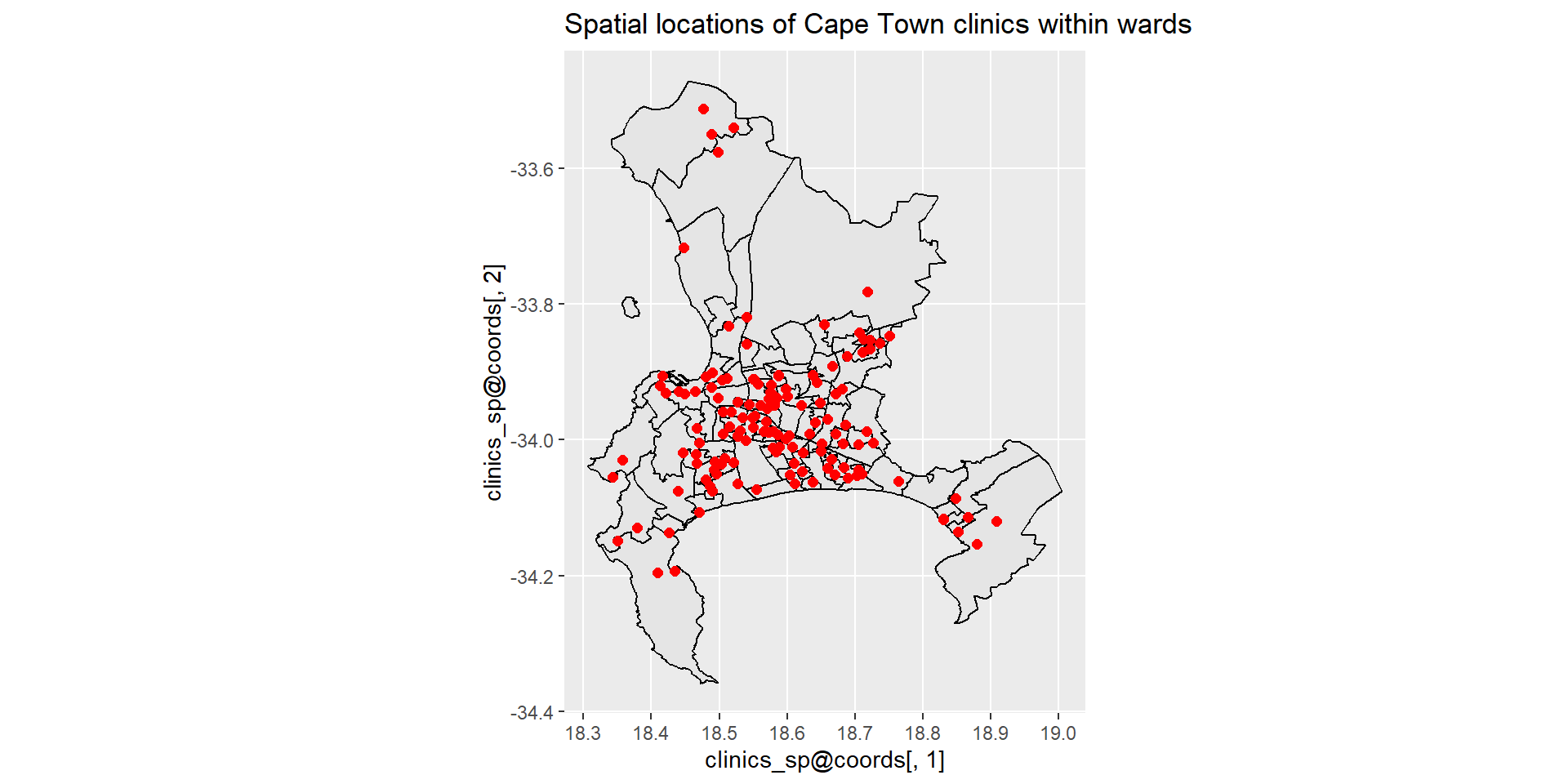

A word of caution on practical data analysis

One of the main aims of this course is to put you in a position of being able to perform the multivariate statistical analysis of your own research projects, in whatever field this may be. Most of the examples used in these notes are themselves real-world studies, and so you will get some idea of some of the complexities involved in gathering and analysing data. Having said that, there is an obvious need in an introductory course like this one to choose data sets that work’ and that can be used to illustrate the techniques. We therefore do not discuss many of the practical difficulties which inevitably arise when doing your own original research. As a result when these difficulties arise when it comes to doing your own research, you may look back on this course and think why weren’t we taught that?’ Unfortunately, the kinds of problems that can arise are so varied and require such different solutions that it is not possible to teach in a course such as this one. As Bartholemew et al. put it, only when one has a clear idea of where one is going is it possible to know the important questions which arise”. However, the following broad areas should be borne in mind whenever conducting an original analysis.

Missing Data

Missing data can cause severe problems for many of the techniques we will consider. Most techniques will simply drop cases which possess missing data on any of the variables to be included in the analysis. When the number of variables is large, as is often the case in multivariate analyses, this can result in a substantial proportion of the sample being dropped. This proportion should always be noted early in the analysis. Another critical question to ask iswhy is the data missing?” and ’does the missing data introduce any bias into the results?” Often, it is the people with the most extreme views that turn up as missing data by refusing to answer certain questions, which is clearly biasing. Possible solutions are mean replacement or other imputation (replacement) techniques, but these are beyond the scope of this course.

Sample Sizes

It is a general rule that the bigger the model you fit, the greater the number of cases you need. In univariate analysis and simple hypothesis testing, the calculation ofrequired’

sample sizes is reasonably straightforward, but in multivariate analysis there are only very rough guidelines where any exist at all. As a very rough guideline, most techniques require at least 10 respondents per parameter estimated. That means that in order to estimate a regression model with four independent variable, you need at least 50 respondents (not forgetting the constant term \(\beta_0\), there are 5 parameters to be estimated). When sample sizes are small, one should be very careful about drawing strong conclusions. This is a particular problem in student research, where sample sizes are typically very small.

Transformations

Many statistical techniques assume that data are normally distributed. Although it is again beyond the scope of this course, it is often possible to transform data that is not normally distributed into something that is normally distributed by using some kind of transforming function. Taking the logarithm of a set of numbers, for example, often works, as does taking the square (both of these transformations work by sucking in’ the tails of the non-normal distributions). Where transformations do not help, the analyst must make a decision about whether the data is approximately normal’ or ‘normal enough’ to continue, or whether it is necessary to use other methods (like non-parametric statistics, which tend to be harder to use but do not make any distributional assumptions).